Continuous Probability Distributions

1. Continuous Probability Distributions Statistics for Management and Economics Chapter 8

2. Probability Density Functions • Unlike a discrete random variable which we studied in Chapter 7, a continuous random variable is one that can assume an uncountable number of values. •  We cannot list the possible values because there is an infinite number of them. •  Because there is an infinite number of values, the probability of each individual value is virtually 0.

3. Point Probabilities are Zero • Because there is an infinite number of values, the probability of each individual value is virtually 0. • Thus, we can determine the probability of a range of values only. • E.g. with a discrete random variable like tossing a die, it is meaningful to talk about P(X=5), say. • In a continuous setting (e.g. with time as a random variable), the probability the random variable of interest, say task length, takes exactly 5 minutes is infinitesimally small, hence P(X=5) = 0. It is meaningful to talk about P(X ≤ 5).

4. f(x) area=1 a b x Probability Density Function A function f(x) is called a probability density function (over the range a ≤ x ≤ b if it meets the following requirements: • f(x) ≥ 0 for all x between a and b, and • The total area under the curve between a and b is 1.0

5. Characteristics of Density Functions All density functions must satisfy the following two requirements: • The curve must never fall below the horizontal axis. That is,f(x) ≥ 0 for all x • The total area between the curve and the horizontal axis must be 1. In calculus this is expressed as: f(x) dx = 1

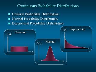
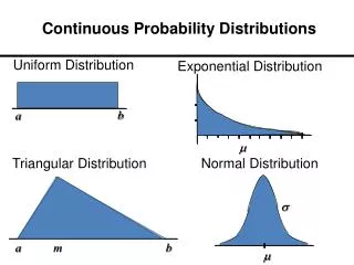
6. f(x) a b x area = width x height = (b – a) x = 1 Uniform Distribution • Consider the uniform probability distribution (sometimes called the rectangular probability distribution). • It is described by the function: *f(x) = 0 for all other values

7. The Normal Distribution • The normal distribution is the most important of all probability distributions. The probability density function of a normal random variable is given by: • It looks like this: • Bell shaped, • Symmetrical around the mean

8. The Normal Distribution The normal distribution is fully defined by two parameters: its standard deviation andmean The normal distribution is bell shaped and symmetrical about the mean Unlike the range of the uniform distribution (a ≤ x ≤ b) Normal distributions range from minus infinity to plus infinity

9. 0 1 1 Standard Normal Distribution • A normal distribution whose mean is zero and standard deviation is one is called the standard normal distribution. • As we shall see shortly, any normal distribution can be converted to a standard normal distribution with simple algebra. This makes calculations much easier.

10. Normal Distribution The normal distribution is described by two parameters: Its mean and its standard deviation . Increasing the mean shifts the curve to the right…

11. Normal Distribution The normal distribution is described by two parameters: its mean and its standard deviation . Increasing the standard deviation “flattens” the curve…

12. Calculating Normal Probabilities We can use the following function to convert any normal random variable to a standard normal random variable… 0 Some advice: always draw a picture!

13. Calculating Normal Probabilities We can use the following function to convert any normal random variable to a standard normal random variable… 0 This shifts the mean of X to zero…

14. Calculating Normal Probabilities We can use the following function to convert any normal random variable to a standard normal random variable… 0 This changes the shape of the curve…

15. Calculating Normal Probabilities We can use Table 3 in Appendix B to look-up probabilities P(0 < Z < z) We can break up P(–.5 < Z < 1) into: P(–.5 < Z < 0) + P(0 < Z < 1) The distribution is symmetric around zero, so (multiplying through by minus one and re-arranging the terms) we have: P(–.5 < Z < 0) = P(.5 > Z > 0) = P(0 < Z < .5) Hence: P(–.5 < Z < 1) = P(0 < Z < .5) + P(0 < Z < 1)

16. Calculating Normal Probabilities How to use Table 3… This table gives probabilities P(0 < Z < z) First column = integer + first decimal Top row = second decimal place P(0 < Z < 0.5) P(0 < Z < 1) P(–.5 < Z < 1) = .1915 + .3414 = .5328

17. Calculating Normal Probabilities • Recap: The time required to build a computer is normally distributed with a mean of 50 minutes and a standard deviation of 10 minutes • What is the probability that a computer is assembled in a time between 45 and 60 minutes? • P(45 < X < 60) = P(–.5 < Z < 1) = .5328 • “Just over half the time, 53% or so, a computer will have an assembly time between 45 minutes and 1 hour”

18. Using the Normal Table What is P(Z > 1.6) ? P(0 < Z < 1.6) = .4452 z 0 1.6 P(Z > 1.6) = .5 – P(0 < Z < 1.6) = .5 – .4452 = .0548

19. Using the Normal Table P(0 < Z < 2.23) What is P(Z < -2.23) ? P(Z < -2.23) P(Z > 2.23) z 0 -2.23 2.23 P(Z < -2.23) = P(Z > 2.23) = .5 – P(0 < Z < 2.23) = .0129

20. Using the Normal Table What is P(Z < 1.52) ? P(0 < Z < 1.52) P(Z < 0) = .5 z 0 1.52 P(Z < 1.52) = .5 + P(0 < Z < 1.52) = .5 + .4357 = .9357

21. Using the Normal Table P(0 < Z < 0.9) What is P(0.9 < Z < 1.9) ? P(0.9 < Z < 1.9) z 0 0.9 1.9 P(0.9 < Z < 1.9) = P(0 < Z < 1.9) – P(0 < Z < 0.9) =.4713 – .3159 = .1554

22. Finding Values of Z Often we’re asked to find some value of Z for a given probability, i.e. given an area (A) under the curve, what is the corresponding value of z (zA) on the horizontal axis that gives us this area? That is: P(Z > zA) = A

23. Area = .50 Area = .025 Area = .50–.025 = .4750 Finding Values of Z What value of z corresponds to an area under the curve of 2.5%? That is, what is z.025 ? If you do a “reverse look-up” on Table 3 for .4750,you will get the corresponding zA = 1.96 Since P(z > 1.96) = .025, we say: z.025 = 1.96

24. Finding and Using Values of Z • Excel can be used to find values for normally distributed variables. • Syntax: NORMDIST(x,mean,standard_dev,cumulative) • Returns the normal distribution for the specified mean and standard deviation. • X is the value for which you want the distribution. • Mean is the arithmetic mean of the distribution. • Standard_dev is the standard deviation of the distribution. • Cumulative is a logical value that determines the form of the function. If cumulative is TRUE, NORMDIST returns the cumulative distribution function; if FALSE, it returns the probability mass function. • Syntax: NORMSDIST(z) • Z is the value for which you want the distribution. • Returns the standard normal cumulative distribution function. The distribution has a mean of 0 (zero) and a standard deviation of one. Use this function in place of a table of standard normal curve areas.

25. Finding and Using Values of Z • Other Z values are • Z.05 = 1.645 • Z.01 = 2.33 • Because z.025 = 1.96 and - z.025= -1.96, it follows that we can state P(-1.96 < Z < 1.96) = .95 • Similarly, P(-1.645 < Z < 1.645) = .90

26. Exponential Distribution • Another important continuous distribution is the exponential distribution • Closely related to the discrete Poisson distribution • Describes a probability distribution of the times between random occurrences • Skewed to the right • The x values range from zero to infinity • Curve steadily decreases as x gets larger • The apex (top of the curve) is always at x=0

27. Exponential Distribution • The exponential distribution has this probability density function: • Note that x ≥ 0. Time (for example) is a non-negative quantity; the exponential distribution is often used for time related phenomena such as the length of time between phone calls or between parts arriving at an assembly station. • Note also that the mean and standard deviation are equal to each other and to the inverse of the parameter of the distribution (lambda )

28. Exponential Distribution • The exponential distribution depends upon the value of • Smaller values of “flatten” the curve: • (E.g. exponential distributions for = .5, 1, 2)

29. Exponential Distribution Recall from calculus that, in order to find the area under the curve, we take the integral of the probability density function over all real values of x, f(x) = e-  x . If X is an exponential random variable, then we can calculate probabilities by: f(x) = e - x P(x ≥ x0) = e - x And…

30. Exponential Distribution • Excel can be used to find probabilities for the exponential distribution • Syntax: EXPONDIST(x,lambda,cumulative) • X is the value of the function. • Lambda is the parameter value. • Cumulative is a logical value that indicates which form of the exponential function to provide. If cumulative is TRUE, EXPONDIST returns the cumulative distribution function; if FALSE, it returns the probability density function. • Returns the exponential distribution.

31. Other Continuous Distributions • There are three other important continuous distributions which will be used extensively in later sections: • Student’s t Distribution • Chi-Squared Distribution • F Distribution

32. Student t Distribution • Much like the standard normal distribution, the Student t distribution is bell-shaped and symmetrical about its mean of zero. • In much the same way that  and  define the normal distribution, , the degrees of freedom, defines the Student t Distribution: • As the number of degrees of freedom increases, the t distribution approaches the standard normal distribution.

33. 2Chi-Squared Distribution • Positively skewed continuous distribution • As before, based on , the number of degrees of freedom.

34. F Distribution • F > 0. Two parameters define this distribution, and like we’ve already seen these are again degrees of freedom (df). • 1 is the “numerator” degrees of freedom and 2 is the “denominator” degrees of freedom. • The F distribution is similar to the 2 distribution in that its starts at zero (is non-negative) and is not symmetrical.