Continuous Probability Distributions
Learn about the bell-shaped distribution of continuous random variables, finding Z-values, assessing normality with probability plots, and estimating population parameters using sampling distributions.


Continuous Probability Distributions
E N D
Presentation Transcript
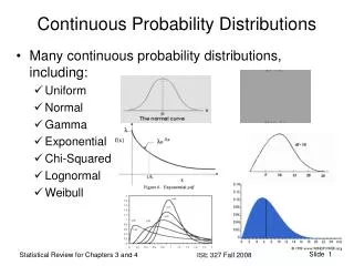
Continuous Probability Distributions • Continuous Random Variable: • Values from Interval of Numbers • Absence of Gaps • Continuous Probability Distribution: • Distribution of a Continuous Variable • Most Important Continuous Probability • Distribution: theNormal Distribution
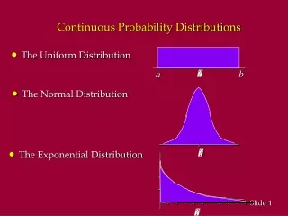
The Normal Distribution • ‘Bell Shaped’ • Symmetrical • Mean, Median and • Mode are Equal • Random Variable has • Infinite Range f(X) X m Mean Median Mode
The Mathematical Model 2 (-1/2) ((X- m)/s) 1 e f(X) = f(X) = frequency of random variable X p = 3.14159; e = 2.71828 s= population standard deviation X= value of random variable (-¥ < X < ¥) m= population mean
Many Normal Distributions There are an Infinite Number Varying the Parameterssandm, we obtainDifferent NormalDistributions.
Which Table? Each distribution has its own table? Infinitely Many Normal Distributions Means Infinitely Many Tables to Look Up!
The Standardized Normal Distribution Standardized Normal Probability Table (Portion) m = 0 and s = 1 Z Z .0478 .02 Z .00 .01 .0000 0.0 .0040 .0080 .0398 .0438 .0478 0.1 0.2 .0793 .0832 .0871 Z = 0.12 0.3 .0179 .0217 .0255 Shaded Area Exaggerated Probabilities
Standardizing Example Normal Distribution Standardized Normal Distribution = 10 s s = 1 Z m 6.2 = 5 m = 0 .12 Z X Shaded Area Exaggerated
Example:P(2.9 < X < 7.1) = .1664 Normal Distribution Standardized Normal Distribution s = 10 s = 1 .1664 .0832 .0832 Z 2.9 5 7.1 X -.21 0 .21 Shaded Area Exaggerated
Example: P(X³ 8) = .3821 . Normal Distribution Standardized Normal Distribution s = 10 s = 1 .5000 .3821 .1179 m = 0 .30 Z m = 5 8 X Shaded Area Exaggerated
Finding Z Values for Known Probabilities What Is Z Given P(Z) = 0.1217? Standardized Normal Probability Table (Portion) .01 s = 1 Z .00 0.2 .1217 0.0 .0040 .0000 .0080 0.1 .0398 .0438 .0478 0.2 .0793 .0832 .0871 m = 0 .31 Z .1179 .1255 .1217 0.3 Shaded Area Exaggerated
Finding X Values for Known Probabilities Normal Distribution Standardized Normal Distribution s = 10 s = 1 .1217 .1217 ? m = 0 .31 Z m = 5 X X 8.1 = m + Zs = 5 + (0.31)(10) = Shaded Area Exaggerated
Assessing Normality • Compare Data Characteristics • to Properties of Normal • Distribution • Put Data into Ordered Array • Find Corresponding Standard • Normal Quantile Values • Plot Pairs of Points • Assess by Line Shape Normal Probability Plot for Normal Distribution 90 X 60 Z 30 -2 -1 0 1 2 Look for Straight Line!
Normal Probability Plots Left-Skewed Right-Skewed 90 90 X X 60 60 Z Z 30 30 -2 -1 0 1 2 -2 -1 0 1 2 Rectangular U-Shaped 90 90 X X 60 60 Z Z 30 30 -2 -1 0 1 2 -2 -1 0 1 2
Estimation _ • Sample Statistic Estimates Population Parameter • e.g. X = 50 estimates Population Mean, m • Problems: Many samplesprovidemany estimates of the Population Parameter. • Determining adequate sample size: large sample give better estimates. Large samples more costly. • How good is the estimate? • Approach to Solution:Theoretical Basis is Sampling Distribution.
Properties of Summary Measures • Population Mean Equal to • Sampling Mean • The Standard Error (standard deviation) of the Sampling distribution is Less than Population Standard Deviation • Formula (sampling with replacement): s s _ = s _ As n increase,decrease. x x
Central Limit Theorem As Sample Size Gets Large Enough Sampling Distribution Becomes Almost Normal regardless of shape of population
Population Proportions • Categorical variable (e.g., gender) • % population having a characteristic • If two outcomes, binomial distribution • Possess or don’t possess characteristic • Sample proportion (ps)
Sampling Distribution of Proportion • Approximated by normal distribution • n·p³ 5 • n·(1 - p) ³ 5 • Mean • Standard error Sampling Distribution ü P(ps) ü .3 .2 .1 0 ps 0 . 2 .4 .6 8 1 p = population proportion
Standardizing Sampling Distribution of Proportion p p - - m p s s Z p @ = s p Sampling Distribution Standardized Normal Distribution sp s = 1 ps Z mp m = 0