Continuous Probability Distributions
Continuous Probability Distributions. Chapter 7. GOALS. Understand the difference between discrete and continuous distributions. Compute the mean and the standard deviation for a uniform distribution . Compute probabilities by using the uniform distribution.


Continuous Probability Distributions
E N D
Presentation Transcript
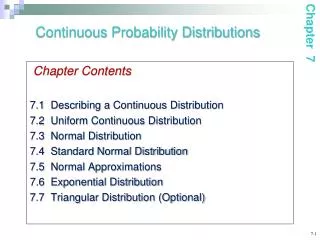
Continuous Probability Distributions Chapter 7
GOALS • Understand the difference between discrete and continuous distributions. • Compute the mean and the standard deviation for a uniform distribution. • Compute probabilities by using the uniform distribution. • List the characteristics of the normal probability distribution. • Define and calculate z values. • Determine the probability an observation is between two points on a normal probability distribution. • Determine the probability an observation is above (or below) a point on a normal probability distribution. • Use the normal probability distribution to approximate the binomial distribution.
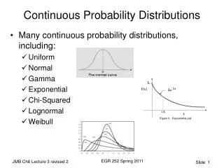
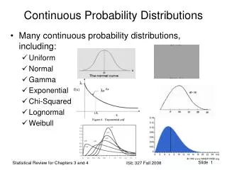
The Uniform Distribution The uniform probability distribution is perhaps the simplest distribution for a continuous random variable. This distribution is rectangular in shape and is defined by minimum and maximum values.
The Uniform Distribution - Example Southwest Arizona State University provides bus service to students while they are on campus. A bus arrives at the North Main Street and College Drive stop every 30 minutes between 6 A.M. and 11 P.M. during weekdays. Students arrive at the bus stop at random times. The time that a student waits is uniformly distributed from 0 to 30 minutes. • Draw a graph of this distribution. • Show that the area of this uniform distribution is 1.00. • How long will a student “typically” have to wait for a bus? In other words what is the mean waiting time? What is the standard deviation of the waiting times? • What is the probability a student will wait more than 25 minutes • What is the probability a student will wait between 10 and 20 minutes?
The Uniform Distribution - Example 1. Draw a graph of this distribution.
The Uniform Distribution - Example 2. Show that the area of this distribution is 1.00
The Uniform Distribution - Example 3. How long will a student “typically” have to wait for a bus? In other words what is the mean waiting time? What is the standard deviation of the waiting times?
The Uniform Distribution - Example 4. What is the probability a student will wait more than 25 minutes?
The Uniform Distribution - Example 5. What is the probability a student will wait between 10 and 20 minutes?
Characteristics of a Normal Probability Distribution • It is bell-shaped and has a single peak at the center of the distribution. • It is symmetricalabout the mean • It is asymptotic: The curve gets closer and closer to the X-axis but never actually touches it. To put it another way, the tails of the curve extend indefinitely in both directions. • The location of a normal distribution is determined by the mean,, the dispersion or spread of the distribution is determined by the standard deviation,σ . • The arithmetic mean, median, and mode are equal • The total area under the curve is 1.00; half the area under the normal curve is to the right of this center point and the other half to the left of it
The Family of Normal Distribution Different Means and Standard Deviations Equal Means and Different Standard Deviations Different Means and Equal Standard Deviations
The Standard Normal Probability Distribution • The standard normal distribution is a normal distribution with a mean of 0 and a standard deviation of 1. • It is also called the z distribution. • A z-value is the signed distance between a selected value, designated X, and the population mean , divided by the population standard deviation, σ. • The formula is:
The Normal Distribution – Example The weekly incomes of shift foremen in the glass industry follow the normal probability distribution with a mean of $1,000 and a standard deviation of $100. What is the z value for the income, let’s call it X, of a foreman who earns $1,100 per week? For a foreman who earns $900 per week?
The Empirical Rule • About 68 percent of the area under the normal curve is within one standard deviation of the mean. • About 95 percent is within two standard deviations of the mean. • Practically all is within three standard deviations of the mean.
The Empirical Rule - Example As part of its quality assurance program, the Autolite Battery Company conducts tests on battery life. For a particular D-cell alkaline battery, the mean life is 19 hours. The useful life of the battery follows a normal distribution with a standard deviation of 1.2 hours. Answer the following questions. • About 68 percent of the batteries failed between what two values? • About 95 percent of the batteries failed between what two values? • Virtually all of the batteries failed between what two values?
Normal Distribution – Finding Probabilities In an earlier example we reported that the mean weekly income of a shift foreman in the glass industry is normally distributed with a mean of $1,000 and a standard deviation of $100. What is the likelihood of selecting a foreman whose weekly income is between $1,000 and $1,100?
Finding Areas for Z Using Excel The Excel function =NORMDIST(x,Mean,Standard_dev,Cumu) =NORMDIST(1100,1000,100,true) generates area (probability) from Z=1 and below
Normal Distribution – Finding Probabilities (Example 2) Refer to the information regarding the weekly income of shift foremen in the glass industry. The distribution of weekly incomes follows the normal probability distribution with a mean of $1,000 and a standard deviation of $100. What is the probability of selecting a shift foreman in the glass industry whose income is: Between $790 and $1,000?
Normal Distribution – Finding Probabilities (Example 3) Refer to the information regarding the weekly income of shift foremen in the glass industry. The distribution of weekly incomes follows the normal probability distribution with a mean of $1,000 and a standard deviation of $100. What is the probability of selecting a shift foreman in the glass industry whose income is: Less than $790?
Normal Distribution – Finding Probabilities (Example 4) Refer to the information regarding the weekly income of shift foremen in the glass industry. The distribution of weekly incomes follows the normal probability distribution with a mean of $1,000 and a standard deviation of $100. What is the probability of selecting a shift foreman in the glass industry whose income is: Between $840 and $1,200?
Normal Distribution – Finding Probabilities (Example 5) Refer to the information regarding the weekly income of shift foremen in the glass industry. The distribution of weekly incomes follows the normal probability distribution with a mean of $1,000 and a standard deviation of $100. What is the probability of selecting a shift foreman in the glass industry whose income is: Between $1,150 and $1,250
Using Z in Finding X Given Area - Example Layton Tire and Rubber Company wishes to set a minimum mileage guarantee on its new MX100 tire. Tests reveal the mean mileage is 67,900 with a standard deviation of 2,050 miles and that the distribution of miles follows the normal probability distribution. Layton wants to set the minimum guaranteed mileage so that no more than 4 percent of the tires will have to be replaced. What minimum guaranteed mileage should Layton announce?
Normal Approximation to the Binomial • The normal distribution (a continuous distribution) yields a good approximation of the binomial distribution (a discrete distribution) for large values of n. • The normal probability distribution is generally a good approximation to the binomial probability distribution when n and n(1- ) are both greater than 5.
Normal Approximation to the Binomial Using the normal distribution (a continuous distribution) as a substitute for a binomial distribution (a discrete distribution) for large values of n seems reasonable because, as n increases, a binomial distribution gets closer and closer to a normal distribution.
Continuity Correction Factor The value .5 subtracted or added, depending on the problem, to a selected value when a binomial probability distribution (a discrete probability distribution) is being approximated by a continuous probability distribution (the normal distribution).
How to Apply the Correction Factor Only one of four cases may arise: • For the probability at least X occurs, use the area above (X -.5). 2. For the probability that more than X occurs, use the area above (X+.5). 3. For the probability that X or fewer occurs, use the area below (X -.5). 4. For the probability that fewer than X occurs, use the area below (X+.5).
Normal Approximation to the Binomial - Example Suppose the management of the Santoni Pizza Restaurant found that 70 percent of its new customers return for another meal. For a week in which 80 new (first-time) customers dined at Santoni’s, what is the probability that 60 or more will return for another meal?
P(X ≥ 60) = 0.063+0.048+ … + 0.001) = 0.197 Normal Approximation to the Binomial - Example Binomial distribution solution:
Normal Approximation to the Binomial - Example Step 1. Find the mean and the variance of a binomial distribution and find the z corresponding to an X of 59.5 (x-.5, the correction factor) Step 2: Determine the area from 59.5 and beyond