Mastering Spreadsheet Basics: Data Organization and Formulas
This guide explains fundamental concepts of spreadsheet usage, focusing on how data is organized within rows, columns, and cell ranges. You will learn the difference between relative and absolute references, and how to apply these concepts when creating and filling formulas. The document also covers arranging information into lists, sorting data, and applying formatting to enhance data presentation. Additionally, you will discover how to use cell addresses to create dynamic formulas that automatically update. Perfect for beginners and anyone looking to improve their spreadsheet skills.


Mastering Spreadsheet Basics: Data Organization and Formulas
E N D
Presentation Transcript
Learning Objectives • Explain how data is organized in spreadsheets • Describe how to refer to spreadsheet rows, columns, and cell ranges • Explain relative and absolute references • Apply concepts of relative and absolute references when filling a formula • Explain the concept of tab-delimited input and output
Arranging Information • Frequently, textual information is organized into lists: • shopping lists • invitation lists • “to do” lists • class lists • Computers don’t have your knowledge about how big the list is • Separate lines help the computer get it
An Array of Cells • Spreadsheets give us an array of cells for setting up a list • The lines are part of the GUI • They help the computer and us agree on: • What an item is • How the positions of items are related to each other
An Array of Cells • Four of the six items do not fit within the lines provided • Entries do not straddle cells • Each item occupies only the cell in which itis typed • Items only spill when the cells to their right are unused • We can either let the entries be clipped or make the cells wider
Sorting the Data • A common operation on any list is to alphabetize or sort it • We must specify which items to sort • Select the list by dragging the cursor across the cells • Resulting selection is indicated with highlighting
Sorting the Data • All of the items are selected (including the white item) • The item is a different color only because it was the first cell selected • The Sort operation is either among the menu items or is an icon • Sorting can be either ascending or descending
Sorting the Data • The sorting software orders the list alphabetically on the first letter of the entry • The spreadsheet views that the cell entries are “atomic” or “monolithic”
Adding More Data to the List • Spreadsheets give us the ability to format cell entries with the kinds of formatting found in word processors: • italics, bold, fontstyles, font sizes,justification, colored text and so on • Formatting facilities are frequently found under the Format menu
Naming Rows and Columns • If the whole list is highlighted, how do we specify which column should be sorted? • Spreadsheet programs automatically provide a naming scheme for referring to specific cells • Columns are labeled with letters and the rows are labeled with numbers
Naming Rows and Columns • This allows us to refer to a: • whole column by its letter • entire row by its number
Naming Rows and Columns • The naming scheme allows a group of cells to be referenced: • Naming the first cell and the last cell and placing a colon (:) • Example: B2:D7 is called a cell range
Headings • It is convenient to name the rows and columns with more meaningful names by giving them headings
Spreadsheet Summary • Spreadsheets are formed from cells that are displayed as rectangles in a grid • Information entered in a cell is treated as an elemental piece of data • A list of items that can be sorted • Spreadsheets provide a labeling for specifying the column/row
Computing with Spreadsheets • Spreadsheets don’t have to contain a single number to be useful • Their most common application is to process numerical data • Numerical data is usually associated with textual information so most spreadsheets allow both
Writing a Formula • First, decide what you want to calculate • Are the values in a particular cell (such as F2) • Within a cell: • Begin a formula with a = (equals sign) • Type a cell address (or click it) • Enter the math operand and any numbers that may be involved=F2 * 0.621
Writing a Formula • Using a cell address (F2) in a formula means that if the value in F2 ever changes, then the value (in H2) automatically changes • H2 holds a formula, not text or a number • H2 is actually: H2 = F2 * 0.641
Repeating a Formula • Similar computations can be done for other cells in that column: • Enter them in the same way as you entered the first formula • Copy/Paste • Don’t worry, it does NOT copy the formula exactly! • Filling “pulls” the formula into other cells
Copy/Paste • When a cell is selected in Excel, it is indicated by an animated highlight (the dashes revolve around the box) • Other spreadsheet software simply shows a solid box around the item. • The cell’s contents are shown in the Edit Formula window • Copy this cell, select the remaining cells in the column by dragging the mouse across them, and Paste (^V)
Copy/Paste • Check the result in the cell. • The original cell had the formula: F2 * 0.621 • The new cell has the formula: F3 * 0.621 • This • The formula was transformed into F3*0.621 when it was pasted
Filling • Filling is another way to copy information, including formulas, to another cell • Notice the small box or tab in the cell’s lower-right corner • This is the fill handle
Filling • When the handle is grabbed, it becomes a + • Pull the handle down the column (or across a row) • This process is known as filling • It automates copying and pasting
Transforming Formulas: Relative Versus Absolute • The spreadsheet software automatically transforms the formulas as it pastes/fills them into a cell • The cell contains a relativecell reference (F2) • Spreadsheets allow two kinds of cell references—relative and absolute • The absolutecellreference to this cell is $F$2
Relative Versus Absolute • Relative means “relative position from a cell” • In the formula H2 =F2*0.621 into H2, the software noticed that cell F2 is two cells to the left of H2 • The formula refers to a cell in the same row, but two cells to the left • This is a relative reference
Relative Versus Absolute • Absolute references always refer to a fixed position—the software never adjusts it • There are two ways a formula can be relative, making four cases: • F2—column and row are both relative • $F2—absolute column, but relative row • F$2—relative column, but absolute row • $F$2—column and row are both absolute
Cell Formats • The scores are somewhat difficult to read because they have too many digits • All spreadsheet software provides control over formatting
Cell Formats • This GUI gives us control over: • The types of information in the fields (Category) • The number of decimal digits for the Number category chosen • Setting the “1000s” separators (commas for North America) • The display of negative numbers
Functions • Spreadsheet software provides functions for computing common summary operations • totals (sum), averages, maximums (max), and others • To use these functions, give the function name and specify the cell range to be summarized in parentheses after it: =max(J2:J7)
Functions • There is a full list of function names under Insert > Insert Function. . . . • A computation value inherits the formatting of the cell • When the function is then dragged across to other columns,it brings its formatting with it
Displaying Hidden Columns • Notice the hidden columns between B and F • When we “unhide” these columns, we have the final spreadsheet
Filling Hidden Columns • Notice the hidden columns between G and J • When we “unhide” these columns, we have computed the maximum and average of the hidden columns
Charts • Spreadsheets organize our data and compute new values • It is helpful to see the results graphically when comparing values • Spreadsheet software makes creating charts easy • Select the values to be plotted and then click Chart
Charts • There are choices of graph styles: • The software detects that the column has a heading and uses it as a label the point as a key to the right • Clicking (or right-click) on any part of the graph, gets a pop-up window that offers editing options
Daily Spreadsheets • Spreadsheets are convenient, versatile tools that simplify computing • Here are some ways to use spreadsheets to organize: • Track our performance in our exercise program • Set up an expense budget • Keep a list of books and DVDs we’ve lent • Follow our favorite team’s successes • Save records generated while online banking • Address books
Solving a Problem of Personal Interest • Scenario: • Time Zone Cheat Sheet • People you want to chat with live in different time zone • It’s not always convenient to chat when you want to call because they may be sleeping, working, or studying
Series Fill • There is certain data that are “special:” days, dates, and time • When the software fills these values, it automatically increments them • Adding 1 to Sunday results in Monday • Adding 1 to January 31 results in February 1 • Adding 1 to 12:00 am produces 1:00 pm • However, if you type Sunday and want Sunday, use Copy/Paste
Series Fill • The best way to use series fill is to: • Enter the first two items of the series into adjacent cells • Select the two cells • Pull on the handle to fill either the row or column • The double-cell fill indicates a series where increment between successive items is the difference between them
Getting Started… • Begin by placing the headings at the top • Under your name enter midnight • Fill down the column to the end of the day • Next, add the times in for your friends • Grab the fill handle and fill the column up and down • The software assumes that rows above are earlier and rows below are later