Download

1 / 31
340 likes | 1.55k Vues
Numerical Solution of Differential Equations. Matlab Tutorial 3. Introduction. MATLAB has several routines for numerical integration ode45, ode 23, ode 113, ode 15s, ode 23s, etc. Here we will introduce two of them: ode45 and ode23

E N D
Numerical Solution of Differential Equations Matlab Tutorial 3
Introduction • MATLAB has several routines for numerical integration ode45, ode23, ode113, ode15s, ode23s, etc. • Here we will introduce two of them: ode45 and ode23 • ode23 uses 2nd-order and ode45 uses 4th-order Runge-Kutta integration. We will learn more about Runge-Kutta method in the class.
Integration by ode23 and ode45: Matlab Command [t, x] = ode45(‘xprime’, [t0,tf], x0) where xprime is a string variable containing the name of the m-file for the derivatives. t0 is the initial time tf is the final time x0 is the initial condition vector for the state variables t a (column) vector of time x an array of state variables as a function of time
Note • We need to generate a m-file containing expressions for differential equations first. • We’ll examine common syntax employed in generating the script or m-file • These objectives will be achieved through 2 examples: • Example-1 on Single-Variable Differential Equation • Example-2 on Multi-Variable Differential Equation
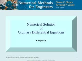
V Example 1: Start-up time of a CSTR Objective: Solve differential mole balance on a CSTR using MATLAB integration routine. Problem description: A CSTR initially filled in 2mol/L of A is to be started up with specified conditions of inlet concentration, inlet and outlet flow rates. The reactor volume and fluid density is considered to be constant. Refer to Module3b classnotes for more details. Reaction: A → B Rate Kinetics: (-rA) = kCA Initial Condition: at t=0, CA = CA,initial = 2 mol/L
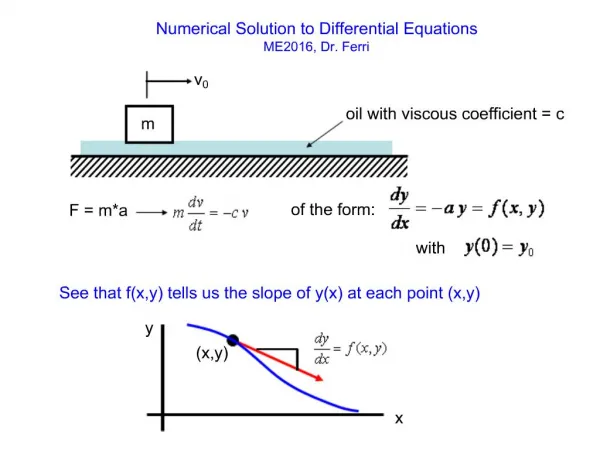
Example 1 The following first-order differential equation in single-variable (CA) is obtained from mole balance on A: Recall, that mass balance yields
generating a m-file titled cstr.m function dx=cstr (t, x) % define constants k=0.005; %mol/L-s V=10; % Reactor volume in L vin=0.15; % Inlet volumetric flow rate in L/s Ca0=10; % Inlet concentration of A in mol/L %For convenience sake, declaring that variable x is Ca Ca=x %define differential equation dx=(vin/V)*Ca0-(vin/V+k)*Ca;
Purpose of function files function output=function_name (input1, input2) As indicated above, the function file generates the value of outputs every time it called upon with certain sets of inputs of dependent and independent variables For instance the cstr.m file generates the value of output (dx), every time it is called upon with inputs of independent variable time (t) and dependent variable (x) NOTE: For cstr.m file, the output dx is actually dCa/dt and x is equal to Ca. function dx=cstr (t, x)
Function File: Command Structure function output=function_name (input1, input2) function dx = CSTR (t, x) Define constants (e.g. k, Ca0, etc.) (Optional) Write equations in terms of constants Define differential equations that define outputs (dx=…)
File & Function Name Example: m-file titled cstr.m Function name should match file name function dx=cstr (t, x) % define constants k=0.005; %mol/L-s V=10; % Reactor volume in L
Inputs and Outputs Example: m-file titled cstr.m Inputs are independent variable (t) and dependent variable (x=Ca) Output is differential, dx = dCa/dt function dx=cstr (t, x) % define constants k=0.005; %mol/L-s V=10; % Reactor volume in L
Writing Comments Example: m-file titled cstr.m Any text written after “ % ” symbol is considered to be commented function dx=cstr (t, x) % define constants k=0.005; %mol/L-s V=10; % Reactor volume in L
Semicolon at the end of an expression Example: m-file titled cstr.m function dx=cstr (t, x) % define constants k=0.005; %mol/L-s V=10; % Reactor volume in L Semi-colon simply suppresses SCREEN printing of the expression.
Example-1 • enter the following MATLAB command [t, x]=ode45(‘cstr’,[0 500],[2]’); • to see the transient response, use plot function plot(t, x); Refer to slide-3 for syntax of above command
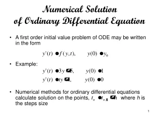
V Example 2: CSTR Response to change in volumetric flow rate. • Objective: Solve differential mole balance on a CSTR using MATLAB integration routine. • Problem description: CSTR operating at SS is subjected to a small disturbance in inlet volumetric flow rate while the outlet volumetric flow rate is kept constant. Both total mass balance and species mole balance must be solved simultaneously. Refer to Module3b class notes for more details.
Example 2 First-order differential equation in two-variables – V(t) and CA(t): Equations (1) and (2) must be solved simultaneously. (1) (2)
Generating the script file dx=cstr1 (t, x) %constant k=0.005; %mol/L-s vout=0.15; % L/s Ca0=10; %mol/L % The following expression describe disturbance in input flow rate if(t <=2) vin=0.15+.05*t elseif(t<=4) vin=0.25-0.05*(t-2); else vin=0.15; end % define x1 and x2 V=x(1,:) Ca=x(2,:) % write the differential equation dx(1,:)=vin-vout; dx(2,:)=(vin/V)*(Ca0-Ca)-k*Ca;
Recognizing Multivariable System The first important point to note is that x is a vector of 2 variables, x1 (=V) and x2(=Ca) Also, dx is a vector of two differential equations associated with the 2 variables function dx=cstr1 (t, x) % constant k=0.005; %mol/L-s vout=0.15; % L/s Ca0=10; %mol/L
Defining arrays The value of these variables change as a function of time. This aspect is denoted in MATLAB syntax by defining the variable as an array. Thus variable 1 can be indicated as x(1,:) and variable 2 as x(2,:) For bookkeeping purposes or convenience sake, the two variables are re-defined as follows % define x1 and x2 V=x(1,:) Ca=x(2,:)
Defining differential equations There are two differential equations – dV/dt and dCa/dt – that must be solved. These two equations are represented in vector form as “dx” Two differential equations must be defined. The syntax is shown below % write the differential equation dx(1,:)=vin-vout; dx(2,:)=(vin/V)*(Ca0-Ca)-k*Ca;
Example-2 • enter the following MATLAB command [t, x]=ode45(‘cstr1’,[0 500],[10 7.5]’); • to see the transient responses, use plot function plot(t, x(:,1); plot(t, x(:,2); Initial conditions for the two variables, i.e. V=10 L and CA=7.5 mol/L at time t=0
Example-2 • Did you spot any problems in the plots? • Do you see any transient response at all? Likely not. • Type the following Matlab commands • [t, x]=ode45('cstr1',[0:0.1:500],[10 ; 7.5]) • Plot x1 and x2. (see command in previous slide)