Random Dispersal in Theoretical Populations
210 likes | 539 Vues
Random Dispersal in Theoretical Populations. By: J.G. Skellam. J.G. Skellam.

Random Dispersal in Theoretical Populations
E N D
Presentation Transcript
Random Dispersal in Theoretical Populations By: J.G. Skellam
J.G. Skellam • “Traditional biology course lay far too much emphasis on the direct acquisition of information. Insufficient attention is given to the interpretation of facts or to the drawing of conclusions from observations and experience. The student is given little opportunity to apply scientific principles to new situations.”
Random? • From the perspective of Skellam the best way to understand the random dispersal amongst populations was by first understanding the principle of random walks. • So as a reminder of what a random walk is: A random process consisting of a sequence of discrete steps of fixed length.
SOmE MoRe Randomness! • Random walks have interesting mathematical properties that vary greatly depending on the dimension in which the walk occurs and whether it is confined to a lattice.
Skellam’s Perspective • With regards to random walks, Skellam proposed the following: • Consider a plane using the Euclidean coordinate system. • In the immediate neighborhood of the origin let there be a particle that tends to leave the origin to gradually form a circular representation of the previous graph.
uuuggg • Now, this might seem to resemble the concept of Brownian Motion of a particle in a viscous substance but here in lies the difference: • “The distribution of the position of a particle of the nth generation with be henceforth”
Even more uuuggg • Skellam’s polar transformation of this particle positioning of n-generations turned out to be the following:
Are we getting anywhere with this? • Alas!! Integrating over θ gives us the radical probability density: • a^2 = the mean-square dispersion per generation analogous with the mean-square velocity in Maxwell’s distribution.
Soooooo? • So from what we have gathered thus far is that an organism or particle with tend to move away from its origin in a semicircular pattern. • From the previous equations we are then able to calculate its probable whereabouts with regards to random distributing.
Interesting.. • “of the population spread out after n-generations that proportion lying outside a circle of radius R is:”
Awww wook at the fuzzy wuzzies • The results of the particle motion can be made applicable to the dispersal of small animals such as worms and snails. • A bug example: • If the random mean square dispersion (RMSD) per minute of a wingless beetle wandering at random is 1 yard ^2 the after a season of 6 months RMSD of the resulting probability distributions is only 500 yards.
The bug example continued… • The probability that after 6 months the beetle wanders more than a mile from the starting point is less than 8 in a million (wow, wonder how he figured that out?). • Without external aid a period of time equivalent to 1000000 seasons would be required to raise RMSD. • Soooo, basically as RMSD increases a great deal the particle or in this case wingless beetle comes a great deal nearer the origin than the farthermost position previously reached.
TIMBER!!! • Skellam makes reference to Reid’s Problem: • “We can clearly establish a rigorous conclusion in the form of an equality provided that we can fix appropriate bounds to various parameters.” • It turns out the problem that is being referred to is having to do with the Oak tree.
Oaky Doky • The oak does not produce accorns until it is sixty or seventy years old and even then it is not mature. • It then produces acorns over a period of several hundred years. • Obviously not all the acorns grow to produce more Oak trees: • Some are – eaten by mammels, fail to germinate, or are simply overshadowed by the larger mature trees.
It seems that only 1% of the seedlings are likely to survive the next three years. • It is also safe to assume that the oak population is no more than 9 million. • We then have R/a < 300 sqrt(log 9,000,000) = 1200. • In the original form of the problem as stated by Reid, R is given as 600 miles
Lastly.. • It then follows that the rootmean square distance of daughter oaks about their parents is greater than ½ a mile and that agents such as small fuzzy wuzzies (aka mammals and birds) played a major role in the dispersal of this population.
Just kidding, I’ve got more!! • Skellam, goes on to explain that many problems on dispersal cannot be formulated unless some law of population growth (in the absence of dispersal) is assumed. • As long as the population is small of shows a natural tendency to decrease, the Malthusian law dN/dt =cN is usually satisfactory. • If the population is not small the Pearl-Verhulst logistic law is more appropriate. • This law may be written in the form: • dN/dt = cN – lN^2
Almost done, really… • “In practice there is rarely sufficient information to construct the contours of population density with accuracy…” • Buuuuuuut here is a well illustrated spread of the muskrat in central Europe since its introduction in 1905. • If we are prepared to accept a boundary as being representative of a theoretical contour, then we must regard the area enclosed by that boundary as an estimate of pi*r^2
Well that’s about it! • So the basic principle that I want to emphasize is that there is random dispersal in theoretical populations, although not apparent it is virtually everywhere so the next time you are keeping an eye on a particle or tree or beetle or muskrat, just think of Skellam and his principles of random dispersal.