Interest Rate Risk
320 likes | 937 Vues
Interest Rate Risk. Chapter 8. Management of Net Interest Income (Table 8.1, page 159). Suppose that the market’s best guess is that future short term rates will equal today’s rates What would happen if a bank posted the following rates? How can the bank manage its risks?.

Interest Rate Risk
E N D
Presentation Transcript
Interest Rate Risk Chapter 8
Management of Net Interest Income (Table 8.1, page 159) • Suppose that the market’s best guess is that future short term rates will equal today’s rates • What would happen if a bank posted the following rates? • How can the bank manage its risks?
Management of Net Interest Income • Most banks have asset-liability management groups to manage interest rate risk • When long term loans are funded with short term deposits interest rate swaps can be used to hedge the interest rate risk • But this does not hedge the liquidity risk
LIBOR Rates and Swap Rates • LIBOR rates are 1-, 3-, 6-, and 12-month borrowing rates for companies that have a AA-rating • Swap Rates are the fixed rates exchanged for floating in an interest rate swap agreement
Understanding Swap Rates • A bank can • Lend to a series AA-rated borrowers for ten successive six month periods • Swap the LIBOR interest received for the five-year swap rate • This shows that the swap rate has the credit risk corresponding to a series of short-term loans to AA-rated borrowers
Extending the LIBOR Curve • Alternative 1: Create a term structure of interest rates showing the rate of interest at which a AA-rated company can borrow for 1, 2, 3 … years • Alternative 2: Use swap rates so that the term structure represents future short term AA borrowing rates • Alternative 2 is the usual approach. It creates the LIBOR/swap term structure of interest rates
Risk-Free Rate • Traders has traditionally assumed that the LIBOR/swap zero curve is the risk-free zero curve • The Treasury curve is about 50 basis points below the LIBOR/swap zero curve • Treasury rates are considered to be artificially low for a variety of regulatory and tax reasons
OIS Rate • LIBOR/swap rates were clearly not “risk-free” during the crisis • As a result there has been a trend toward using overnight indexed swap (OIS) rates as proxies for the risk-free rate instead of LIBOR and swap rates • The OIS rate is the rate swapped for the geometric average of overnight borrowing rates. (In the U.S. the relevant overnight rate is the fed funds rate)
Duration (page 164) • Duration of a bond that provides cash flow ciat time ti is where B is its price and y is its yield (continuously compounded) • This leads to
Calculation of Duration for a 3-year bond paying a coupon 10%. Bond yield=12%. (Table 8.3, page 166)
Duration Continued • When the yield y is expressed with compounding m times per year • The expression is referred to as the “modified duration”
Convexity (Page 168-169) The convexity of a bond is defined as
Portfolios • Duration and convexity can be defined similarly for portfolios of bonds and other interest-rate dependent securities • The duration of a portfolio is the weighted average of the durations of the components of the portfolio. Similarly for convexity.
What Duration and Convexity Measure • Duration measures the effect of a small parallel shift in the yield curve • Duration plus convexity measure the effect of a larger parallel shift in the yield curve • However, they do not measure the effect of non-parallel shifts
Other Measures • Dollar Duration: Product of the portfolio value and its duration • Dollar Convexity: Product of convexity and value of the portfolio
Partial Duration • A partial duration calculates the effect on a portfolio of a change to just one point on the zero curve
Partial Durations Can Be Used to Investigate the Impact of Any Yield Curve Change • Any yield curve change can be defined in terms of changes to individual points on the yield curve • For example, to define a rotation we could change the 1-, 2-, 3-, 4-, 5-, 7, and 10-year maturities by −3e, − 2e, − e, 0, e, 3e, 6e
Combining Partial Durations to Create Rotation in the Yield Curve (Figure 8.5, page 174)
Impact of Rotation • The impact of the rotation on the proportional change in the value of the portfolio in the example is
Alternative approach (Figure 8.6, page 175)Bucket the yield curve and investigate the effect of a small change to each bucket
Principal Components Analysis • Attempts to identify standard shifts (or factors) for the yield curve so that most of the movements that are observed in practice are combinations of the standard shifts
Results (Tables 8.7 and 8.8 on page 176) • The first factor is a roughly parallel shift (90.9% of variance explained) • The second factor is a twist 6.8% of variance explained) • The third factor is a bowing (1.3% of variance explained)
Alternatives for Calculating Multiple Deltas to Reflect Non-Parallel Shifts in Yield Curve • Shift individual points on the yield curve by one basis point (the partial duration approach) • Shift segments of the yield curve by one basis point (the bucketing approach) • Shift quotes on instruments used to calculate the yield curve • Calculate deltas with respect to the shifts given by a principal components analysis.
Gamma for Interest Rates • Gamma has the form where xi and xjare yield curve shifts considered for delta • To avoid too many numbers being produced one possibility is consider only i = j • Another is to consider only parallel shifts in the yield curve and calculate convexity • Another is to consider the first two or three types of shift given by a principal components analysis
Vega for Interest Rates • One possibility is to make the same change to all interest rate implied volatilities. (However implied volatilities for long-dated options change by less than those for short-dated options.) • Another is to do a principal components analysis on implied volatility changes for the instruments that are traded