Stat 31, Section 1, Last Time

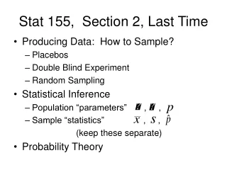
Stat 31, Section 1, Last Time • Foundations of Statistical Inference • Population vs. Samples • Numerical Summaries (mean, SD): • Population: “parameters”, • Sample: “statistics” • Probability: • Numerical Assessment of “uncertainty” • Makes statistics a Quantitative Science

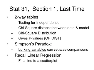
Midterm I Results No grade range given now, since “not enough info…” Recall earlier analyses: Final vs. Midterm I Midterm II vs. Midterm I Final Exam vs. Midterm I Correlation = 0.61 Correlation = 0.57 Correlation = 0.73

Midterm I Results Indicator of Your Status: 90-100 “Very Pleased” 78-89 “OK, but be careful…” 0-77 “Strongly recommend drop course” (or let’s talk…)

Midterm I Results

Pepsi - Coke Results Summary Spreadsheet: https://www.unc.edu/~marron/UNCstat31-2005/Stat31CokePepsiResults2005.xls Prefer Pepsi? 51% Pepsi Sweeter? 53% Think Know? 82% Right? 69% How many Heads? 58% What is “random variation”????

Probability Recall Basics: Assign numbers (representing “how likely”), to outcomes E.g. Die Rolling: P{comes up 4} = 1/6 • Outcome is “4” • Probability is 1/6

Probability - Events More Terminology (to carry this further): • An event is a set of outcomes Die Rolling: “an even #”, is the event {2, 4, 6} Notes: • If betting on even don’t care about #, only even or odd • Thus events are our foundation • Each outcome is an event: the set containing just that outcome • So event is the more general concept

Probability on Events Sample Space is the set of all outcomes = = “event with everything that can happen” Extend Probability to Events by: P{event} = sum of probs of outcomes in event

Probability Technical Summary: • A probability model is a sample space • I.e. set of outcomes, plus a probability, P • P assigns numbers to events, • Events are sets of outcomes

Probability Function The probability, P, is a “function”, defined on a set of events Recall function in math: plug-in get out Probability: P{event} = “how likely”

Probability Function E.g. Die Rolling • Sample Space = {1, 2, 3, 4, 5, 6} • “an even #” is the event {2, 4, 6} (a “set”) • P{“even”} = P{2, 4, 6} = = P{2} + P{4} + P{6} = = 1/6 + 1/6 + 1/6 = 3/6 = ½ • Fits, since expect “even half the time”

Probability HW HW: 4.11 4.13b 4.17 4.19a, b

Probability Now stretch ideas with more interesting e.g. E.g. Political Polls, Simple Random Sampling 2 views: • Each individual equally likely to be in sample • Each possible sample is equally likely Allows for simple Probability Modelling

Simple Random Sampling • Sample Space is set of all possible samples • An Event is a set of some samples E.g. For population A, B, C, D • Each is a voter • Only 4, so easy to work out

S. R. S. Example For population A, B, C, D, Draw a S. R. S. of size 2 Sample Space = {(A,B), (A,C), (A,D), (B,C), (B,D), (C,D)} outcomes, i.e. possible samples of size 2

S. R. S. Example Now assign P, using “equally likely” rule: P{A,B} = P{A,C} = … = P{C,D} = = 1/(#samples) = 1/6 An interesting event is: “C in sample” = {(A,C),(B,C),(D,C)} (set of samples with C in them)

S. R. S. Example P{C in sample} = i.e. happens “half the time”. HW: 4.29

Political Polls Example What is your chance of being in a poll of 1000, from S.R.S. out of 200,000,000? (crude estimate of # of U. S. voters) Recall each sample is equally likely so: Problem: this is really big (5,733 digits, too big for easy handling….)

Political Polls Example More careful calculation: Makes sense, since you are “equally likely to be in samples”

And now for something completely different .

Probability • Now have prob. models • But still hard to work with • E.g. prob’s we care about, such as “accuracy estimators”, need better tools • Need to look more deeply

3 Big Rules of Probability • Main idea: calculate “complicated prob’s” • By decomposing events in terms of simple events • Then calculating probs of these • And then using simple rules of prob.

3 Big Rules of Probability Rule I: the not rule: P{not A} = 1 – P{A} Why? E.g. equally likely sample points: And more generally:

The “Not” Rule of Probability Text Book Terminology (sec. 4.2): not A = for “complement” (set theoretic term) (I prefer “not”, since more intuitive)

The “Not” Rule of Probability HW: Rework, using the “not” rule: 4.17b 4.19a,b

3 Big Rules of Probability Rule II: the or rule: P{A or B} = P{A} + P{B} – P{A or B} Why? E.g. equally likely sample points: Helpful Pic:

Big Rules of Probability E.g. Roll a die, Let A = “4 or less” = {1, 2, 3, 4} Let B = “Odd” = {1, 3, 5} Check how rules work by calculating 2 ways: Direct: P{not A} = P{5, 6} = 2/6 = 1/3 By Rule I: P{not A} = 1 – P{A} = 1 – 4/6 = 1/3

The “Or” Rule of Probability A = “4 or less” = {1, 2, 3, 4} B = “Odd” = {1, 3, 5} Check how rule works by calculating 2 ways: Direct: P{A or B} = P{1, 2, 3, 4, 5} = 5/6 By Rule II: P{A or B} = = P{A} + P{B} – P{A or B} = = 4/6 + 3/6 – 2/6 = 5/6 (check!)

The “Or” Rule of Probability • Seems too easy? • Don’t really need rules for these simple things • But they are the key to bigger problems • Such as Simple Random Sampling HW:

The “Or” Rule of Probability • Seems too easy? • Don’t really need rules for these simple things • But they are the key to bigger problems • Such as Simple Random Sampling HW: 4.86 (0.308)

The “Or” Rule of Probability E.g: A college has 60% Women and 40% smokers, and 50% women who don’t smoke. What is the chance that a randomly selected student is either a women or a non-smoker? (seems “>60%”, but twice? Must be < 100%, i.e. must be some overlap…)

College Women – Smokers E.g. P{W or S} = P{W} + P{S} = P{W & S} (choice of letters make easy to work with) = 0.6 + (1 – 0.4) – 0.5 = 0.7 (answer is 70% women or smokers) Note: rules are powerful when used together HW: 4.89

The “Or” Rule of Probability E.g. Events A & B are “mutually exclusive”, i.e. “disjoint”, when P{A & B} = 0 (i.e. no chance of seeing both at same time) Useful Pic: Then: P{A or B} = P{A} + P{B} Text suggest “new rule”, I say “special case”

The “Exclusive Or” Rule HW: 4.18 (0.65, 0.38, 0.62)

Stat 31, Section 1, Last Time