Download
1 / 26
260 likes | 426 Vues
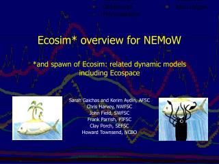
Ecosim* overview for NEMoW *and spawn of Ecosim: related dynamic models including Ecospace. Sarah Gaichas and Kerim Aydin, AFSC Chris Harvey, NWFSC John Field, SWFSC Frank Parrish, PIFSC Clay Porch, SEFSC Howard Townsend, NCBO. What is/has/will the model be used for?.

E N D
Ecosim* overview for NEMoW*and spawn of Ecosim: related dynamic models including Ecospace Sarah Gaichas and Kerim Aydin, AFSC Chris Harvey, NWFSC John Field, SWFSC Frank Parrish, PIFSC Clay Porch, SEFSC Howard Townsend, NCBO
What is/has/will the model be used for? • Describing ecosystems and improving understanding of how simultaneous physical, ecological, and fisheries interactions affect commercial and bycatch species • Examining apex predator (and or protected species) carrying capacity and predicting responses to changing fishing and primary production • Examining ecosystem effects of • changing water quality • changing fishing gear • different MPA scenarios • Evaluating tradeoffs between management strategies • Providing foundation for developing proposals to integrate ecosystem-based management approaches into current management regimes
Has the model been published in the peer reviewed literature? Yes. Early version: Walters, C., Christensen, V., and Pauly, D. 1997. Structuring dynamic models of exploited ecosystems from trophic mass-balance assessments. Rev. Fish. Biol. Fish. 7: 139-172. Most recent version with “multistanza” age structure: Christensen, V., and C. Walters, 2004. Ecopath with Ecosim: methods, capabilities, and limitations. Ecological Modelling 172: 109-139. Ecospace (also covered in Christensen & Walters 04): Walters, C., Pauly, D., and Christensen, V. 1999. Ecospace: prediction of mesoscale spatial patterns in trophic relationships of exploited ecosystems, with emphasis on the impacts of marine protected areas. Ecosystems, 2: 539–554.
Static food web to dynamic simulation requires functional response + age structured population dynamics ?
Hypothetical MPA coverage Where bottom trawling occurs Ecospace: sim in space • Traceable spatial features in grid space • habitats, fleets, ports, management areas, advection fields, seasonal migrations, etc. Habitats (depth, substrate) Columbia River Blanco Mendocino
Biomass dynamics equations • For Biomass of group i, dBi /dt= GEi∑preyQ(BiBprey) consumption gain - FiBifishing loss - M0iBiother mortality loss - ∑predQ(BpredBi) predation loss +I immigration rate
Picturing the “foraging arena” (Walters et al 1997) “It’s cold down there!” Single “vulnerability” parameter X ~ 2v/aBj ratio V dVij /dt= vij(Bi-Vij) - vijVij - aijVijBj B-V Predator Bj Vulnerable prey Vij aijVijBj Assume fast equilibrium for Vij vij (Bi-Vij) vijVij Sophisticated functional response behavior ranges from stable donor-controlled to chaotic Lotka-Volterra Unavailable prey Bi - Vij
Gulf of Alaska (GOA) simulation Low vulnerability versus High vulnerability Biomass (t/km2) Simulation year
The full consumption equation: complex functional response Qt = alinkvlinkBpredBpreyTpredTprey /Dpred vlink + vlinkTprey + alinkBpredTpred / Dpred Where Dpred = hpredTpred 1 + ∑pred’sprey alinkBpreyTprey
Vulnerability: how much prey biomass is available to predators? Foraging Time: if I’m hungry, should I spend more time vulnerable? Handling Time: at some point, my consumption is limited even if there are more prey Functional response parameters “It’s cold down there!” V B-V “Our food is up there, but so are those big guys!” “Don’t worry, I’m still chewing.”
Ecospace equations and assumptions • Same biomass dynamics equation as Ecosim, except with coordinates x, y to designate location on map grid, and movement terms take on greater importance: • Growth efficiency, predation, mortality are now spatially explicit (habitat quality, abundance of other spp., fishing, etc.) • Instantaneous movement mi,x,y reflects organism’s ability to discern fitness trade-offs between x,y and surrounding cells dBi,x,y/dt = GEiSprey Q(Bi,x,yBprey,x,y) consumption gain - Fi,x,yBi,x,yfishing loss - M0iBi,x,yother mortality loss - Spred Q(Bpred,x,yBi,x,y) predation loss + Ii,x,yimmigration gain - mi,x,yBi,x,yemigration loss
Ecospace equations and assumptions • Fishing mortality by fleet k over all N cells of system is equal to N · Fk • For each model time step, that mortality is distributed spatially by assigning a weight G to each cell c: Gkc = Okc · Ukc · Si pkiqkiBic / Ckc Okc = status of fleet k in cell c (0=closed, 1=open) Ukc = ability of fleet k to fish in cell c habitat type (0, 1) pki = price fleet k receives for species i qki = catchability of species i in fleet k Bic = biomass of species i in cell c Ckc = cost for fleet k to operate in cell c
Data requirements I, Ecosim and Ecospace • All food web parameters from Ecopath, plus • Growth information for age structured groups • General habitat preferences • Dispersal and/or migratory characteristics • Time series to “drive” trajectories for some groups • Single species F, and/or Gear specific effort with bycatch • Primary Production or other group production/recruitment, B • Port locations, habitats where fishing occurs • For ecosystem map • Habitat distribution, including land • Advection patterns • 1° production patterns (can use Sea Around Us data) • Location of management zones (statistical areas, MPAs, etc.)
Data requirements II, calibration/fitting • Time series to “fit” (by estimating functional response Vulnerability) • B most common • Species total catch, recruitment • Values for functional response parameters Foraging time, Handling time • Alternatively, estimate these parameters* (see next slides) • Also, include time series of diet data to estimate functional response* • Known species interactions modeled as “mediation functions” • Not available in current version of Ecosim
What key data gaps have been identified? • Many regions missing time series of primary production • Time series that are NOT model output already • Mid TL forage fish and low TL zooplankton group dynamics are key low data interactions in many systems • Often, high TL unexploited predator dynamics (killer whales, seals) are unknown and influential • Nobody really knows functional response parameters Are these data gaps informing monitoring efforts? • Strategic data collections implemented from model gaps at PIFSC • NCBO can inform, but still need money approved • Much other data collection still opportunistic
Experience: equilibrium + uninformative data + vulnerability estimation in the GOA* • Today’s rules (path equilibruim) can’t recreate yesterday’s GOA. Species and or ecosystem production was different historically. • Supports both climate and fishing-related hypotheses for change, but with different predator prey relationships implied by estimated vulnerability parameters *Analyses in Sim alternative
* * * * Different drivers for different species* Key: Lower AIC is better overall fit; Each species fit varies by model Best fit Extinct OK fit
Likelihood and AIC for all models* 250 estimated vul parameters
Even more functional response parameters* Data-free simulation testing using randomly sampled Vul, Ftime, and Htime (324 parameters) gave a wide range of alternative GOA ecosystems
The art part: Pick your poison Too many parameters, not enough data. Options: • The Walters bias: Fix many parameters, fit only vulnerabilities (in blocks), assume systematic residuals are “primary production anomaly.” • The Aydin bias: Group by predator and prey, fit all functional response parameters, assume systematic residuals are difference between start state being “in equilibrium” and the true equilibrium (initial spin-up to “true fitted” equilibrium). • Many other “biases” are possible, and possibly reasonable. Best practice would require more formal evaluation of these hypotheses within a statistical framework. Current EwE software allows only the first hypothesis, “manual adjustment” may be used to achieve the second.
Model improvement: Ecosim equations (re-written) where B* and Q* are biomass and consumption in a reference year (1991) Parameters fit using likelihood criteria to available time series, parallel search algorithms coded in C.
What are the strengths of this model? • Ecosim is freely available, large user community • Improved understanding of data systems (multiple agency, multiple scale data assimilation) • Functional response parameterization is very flexible, much more advanced than many published forms • Simulates a wide variety of fishing scenarios, including spatial management in Ecospace • Simulates changes in production regimes • Ability to represent age structure for many groups • Biomass dynamics of whole ecosystem considered, see both direct effects and side effects of scenarios
What are the weaknesses of this model? • Functional response: • In some cases, results sensitive to (difficult to estimate) functional response parameters • Full functional response flexibility means more parameters to estimate than data available • Model weakness or data weakness??? • True of many stock assessments… • EwE statistical estimation of vulnerability only; manual adjustment of other parameters during calibration difficult to repeat if not well documented • Inability to estimate uncertainty in projections (Sim) • In big models, sensitivity analysis for all parameters is an overwhelming (but necessary) task • Ecospace relatively untested, few published examples
What remains for model development/improvement/enhancement? • More users for Ecospace, comparisons with Atlantis, etc. • Improved data (but when isn’t that the case?) • More rigorous • documentation of parameter estimation process in many applications (e.g. “manual adjustment” vs. statistical fitting) • statistical parameter estimation ability, including fitting to time varying diet composition data • estimation of uncertainty • Direct comparison of outputs with alternative models • Improved compatibility with complementary models • High resolution ocean circulation models • Fishery interaction and management system models • Age structured stock assessments