Formal Semantics
Formal Semantics. Why formalize?. ML is tricky, particularly in corner cases generalizable type variables? polymorphic references? exceptions? Some things are often overlooked for any language evaluation order? side-effects? errors?

Formal Semantics
E N D
Presentation Transcript
Why formalize? • ML is tricky, particularly in corner cases • generalizable type variables? • polymorphic references? • exceptions? • Some things are often overlooked for any language • evaluation order? side-effects? errors? • Therefore, want to formalize what a language's definition really is • Ideally, a clear & unambiguous way to define a language • Programmers & compiler writers can agree on what's supposed to happen, for all programs • Can try to prove rigorously that the language designer got all the corner cases right
Aspects to formalize • Syntax: what's a syntactically well-formed program? • EBNF notation for a context-free grammar • Static semantics: which syntactically well-formed programs are semantically well-formed? which programs type-check? • typing rules, well-formedness judgments • Dynamic semantics: what does a program evaluate to or do when it runs? • operational, denotational, or axiomatic semantics • Metatheory: properties of the formalization itself • E.g. do the static and dynamic semantics match? i.e.,is the static semantics sound w.r.t. the dynamic semantics?
Approach • Formalizing full-sized languages is very hard, tedious • many cases to consider • lots of interacting features • Better: boil full-sized language down into essentialcore, then formalize and study the core • cut out as much complication as possible, without losing the key parts that need formal study • hope that insights gained about core will carry back to full-sized language
The lambda calculus • The essential core of a (functional) programming language • Developed by Alonzo Church in the 1930's • Before computers were invented! • Outline: • Untyped: syntax, dynamic semantics, cool properties • Simply typed: static semantics, soundness, more cool properties • Polymorphic: fancier static semantics
Untyped -calculus: syntax • (Abstract) syntax: e ::= x variable | x. e function/abstraction ( fn x => e) | e1 e2 call/application • Freely parenthesize in concrete syntax to imply the right abstract syntax • The trees described by this grammar are called term trees
Free and bound variables • x. ebindsx in e • An occurrence of a variable x is free in e if it's not bound by some enclosing lambda freeVars(x) x freeVars(x. e) freeVars(e) – {x} freeVars(e1 e2) freeVars(e1) freeVars(e2) • e is closed iff freeVars(e) = {}
-renaming • First semantic property of lambda calculus: bound variables in a term tree can be renamed (properly) without affecting the semantics of the term tree • -equivalent term trees • (x1. x2x1) (x3. x2x3) • cannot rename free variables • terme: e and all -equivalent term trees • Can freely rename bound vars whenever helpful
Evaluation: -reduction • Define what it means to "run" a lambda-calculus program by giving simple reduction/rewriting/simplification rules • "e1 e2" means"e1 evaluates to e2 in one step" • One case: • (x. e1) e2 [xe2]e1 • "if you see a lambda applied to an argument expression, rewrite it into the lambda body where all free occurrences of the formal in the body have been replaced by the argument expression" • Can do this rewrite anywhere inside an expression
Substitution • When doing substitution, must avoid changing the meaning of a variable occurrence [xe]x e [xe]y y, if x y [xe](x. e2) (x. e2) [xe](y. e2) (y. [xe]e2), if x y andy not free in e [xe](e1 e2) ([xe]e1) ([xe]e2) • can use -renaming to ensure "y not free in e"
Result of reduction • To fully evaluate a lambda calculus term, simply perform -reduction until you can't any more • * reflexive, transitive closure of • When you can't any more, you have a value, which is a normal form of the input term • Does every lambda-calculus term have a normal form?
Reduction order • Can have several lambdas applied to an argument in one expression • Each called a redex • Therefore, several possible choices in reduction • Which to choose? Must we do them all? • Does it matter? • To the final result? • To how long it takes to compute? • To whether the result is computed at all?
Two reduction orders • Normal-order reduction(a.k.a. call-by-name, lazy evaluation) • reduce leftmost, outermost redex • Applicative-order reduction(a.k.a. call-by-value, eager evaluation) • reduce leftmost, outermost redexwhose argument is in normal form(i.e., is a value)
e1 e3 e2 e4 Amazing fact #1:Church-Rosser Theorem, Part 1 • Thm. If e1 *e2 and e1 *e3, then e4 such that e2 *e4 and e3 *e4 • Corollary. Every term has a unique normal form, if it has one • No matter what reduction order is used!
Existence of normal forms? • Does every term have a normal form? • Consider: (x. x x) (y. y y)
Amazing fact #2:Church-Rosser Theorem, Part 2 • If a term has a normal form, then normal-order reduction will find it! • Applicative-order reduction might not! • Example: • (x1. (x2. x2)) ((x. x x) (x. x x))
Weak head normal form • What should this evaluate to? (y. (x. x x) (x. x x)) • Normal-order and applicative-order evaluation run forever • But in regular languages, wouldn't evaluate the function's body until we called it • "Head" normal form doesn't evaluate arguments until function expression is a lambda • "Weak" evaluation doesn't evaluate under lambda • With these alternative definitions of reduction: • Reduction terminates on more lambda terms • Correspond more closely to real languages (particularly "weak")
Amazing fact #3:-calculus is Turing-complete! • But the -calculus is too weak, right? • No multiple arguments! • No numbers or arithmetic! • No booleans or if! • No data structures! • No loops or recursion!
Multiple arguments: currying • Encode multiple arguments via curried functions, just as in regular ML (x1, x2). e x1. (x2. e) ( x1x2. e) f(e1, e2) (fe1) e2
Church numerals • Encode natural numbers using stylized lambda terms zero s. z. z one s. z. s z two s. z. s (s z) … n s. z. sn z • A unary encoding using functions • No stranger than binary encoding
Arithmetic on Church numerals • Successor function:take (the encoding of) a number,return (the encoding of) its successor • I.e., add an s to the argument's encoding succ n. s. z. s (n s z) succ zero s. z. s (zero s z)* s. z. s z = one succ two s. z. s (two s z)* s. z. s (s (s z)) = three
Addition • To add x and y, apply succ to yx times • Key idea: x is a function that, given a function and a base, applies the function to the base x times • "a number is as a number does" plus x. y. x succ y plus two three * two succ three * succ (succ three) = five • Multiplication is repeated addition, similarly
Booleans • Key idea: true and false are encoded as functions that do different things to their arguments, i.e., make a choice if b. t. e. b t e true t. e. t false t. e. e if false four six * false four six * six
Combining numerals & booleans • To complete Peano arithmetic, need an isZero predicate • Key idea: call the argument number on a successor function that always returns false (not zero) and a base value that's true (is zero) isZero n. n (x. false) true isZero zero * zero (x. false) true * true isZero two * two (x. false) true * (x. false) ((x. false) true)* false
Data structures • Try to encode simple pairs • Can build more complex data structures out of them • Key idea: a pair is a function that remembers its two input values, and passes them to a client function on demand • First and second are client functions that just return one or the other remembered value mkPair f. s. x. x f s first p. p (f. s. f) second p. p (f. s. s) second (mkPair true four)* second (x. x true four)* (x. x true four) (f. s. s)* (f. s. s) true four * four
Loops and recursion • -calculus can write infinite loops • E.g. (x. x x) (x. x x) • What about useful loops? • I.e., recursive functions? • Ill-defined attempt: fact n.if (isZero n) one (times n (fact (minusnone))) • Recursive reference isn't defined in our simple short-hand notation • We're trying to define what recursion means!
Amazing fact #N: Can define recursive funs non-recursively! • Step 1: replace the bogus self-reference with an explicit argument factG f. n.if (isZero n) one (times n (f (minusnone))) • Step 2: use the paradoxical Y combinator to "tie the knot" fact YfactG • Now all we need is a magic Y that makes its non-recursive argument act like a recursive function…
Y combinator • A definition of Y: Y f. (x. f (x x)) (x. f (x x)) • When applied to a function f: Yf *(x. f (x x)) (x. f (x x)) *f ((x. f (x x)) (x. f (x x))) = f (Y f) *f (f (Y f)) *f (f (f (Y f))) * … • Applies its argument to itself as many times as desired • Computes the "fixed point" of f • Often called fix
Y for factorial fact two *(Y factG)two *factG (Y factG)two *if (isZero two) one (times two ((Y factG) (minustwoone))) *times two ((Y factG)one) *times two (factG (Y factG)one) *times two (if (isZero one) one (times one ((Y factG) (minusoneone)))) *times two (times one ((Y factG)zero)) *times two (times one (factG (Y factG)zero)) *times two (times one (if (isZero zero) one (times zero ((Y factG) (minuszero one))))) *times two (times oneone) * two
Some intuition (?) • Y passes a recursive call of a function to the function • Will lead to infinite reduction, unless one recursive call chooses to ignore its recursive function argument • I.e., have a base case that's not defined recursively • Relies on normal-order evaluation to avoid evaluating the recursive call argument until needed
Summary, so far • Saw untyped -calculus syntax • Saw some rewriting rules, which defined the semantics of -terms • -renaming for changing bound variable names • -reduction for evaluating terms • Normal form when no more evaluation possible • Normal-order vs. applicative-order strategies • Saw some amazing theorems • Saw the power of -calculus to encode lots of higher-level constructs
Simply-typed lambda calculus • Now, let's add static type checking • Extend syntax with types: ::= 1 2 | e ::= x:. e | x | e1 e2 • (The dot is just the base case for types, to stop the recursion. Values of this type will never be invoked, just passed around.)
Typing judgments • Introduce a compact notation for defining typechecking rules • A typing judgment: ├ e : • "In the typing context , expression e has type " • A typing context: a mapping from variables to their types • Syntax: ::= {} | , x :
Typing rules • Give typechecking rule(s) for each kind of expression • Write as a logical inferencerule premise1 … premisen(n 0) ––––––––––––––––– conclusion • Whenever all the premises are true, can deduce that the conclusion is true • If no premises, then called an "axiom" • Each premise and conclusion has the form of a typing judgment
Typing rules forsimply-typed -calculus , x:1 ├ e: 2 ––––––––––––––––––– [T-ABS] ├ (x:1. e) : 1 2 ––––––––––– [T-VAR] ├ x: (x) ├ e1: 2 ├ e2: 2 ––––––––––––––––––––––––– [T-APP] ├ (e1 e2) :
Typing derivations • To prove that a term has a type in some typing context, chain together a tree of instances of the typing rules, leading back to axioms • If can't make a derivation, then something isn't true
Formalizing variable lookup • What does (x) mean? • What if includes several different types for x? = x:, y:, x:, x:, y: • Can this happen? • If it can, what should it mean? • Any of the types is OK? • Just the leftmost? rightmost? • None are OK?
An example • What context is built in the typing derivation for this expression? x:1. (x:2. x) • What should the type of x in the body be? • How should (x) be defined?
Formalizing using judgments ––––––––––––– [T-VAR-1] , x:├ x: ├ x: x y ––––––––––––––– [T-VAR-2] , y:2├ x: • What about the = {} case?
Type-checking self-application • What type should I give to x in this term? x:?. (x x) • What type should I give to the f and x's in Y? Y f:?. (x:?. f (x x)) (x:?. f (x x))
Amazing fact #N+1: All simply-typed -calculus exprs terminate! • Cannot express looping or recursion in simply-typed -calculus • Requires self-application, which requires recursive types, which simply-typed -calculus doesn't have • So all programs are guaranteed to never loop or recur, and terminate in a finite number of reduction steps! • (Simply-typed -calculus could be a good basis for programs that must be guaranteed to finish, e.g. typecheckers, OS packet filters, …)
Adding an explicit recursion operator • Several choices; here's one:add an expression "fix e" • Define its reduction rule: fix e e (fix e) • Define its typing rule: ├ e: –––––––––––––– [T-FIX] ├ (fix e) :
Defining reduction precisely • Use inference rules to define redexes precisely ––––––––––––––––––– [E-ABS] ––––––––––––– [E-FIX] (x:. e1) e2 [xe2]e1fix e e (fix e) e1 e1' e2 e2' ––––––––––––– [E-APP1] ––––––––––––– [E-APP2] e1e2 e1'e2 e1e2 e1e2' e1 e1' ––––––––––––––––– [E-BODY] optional x:. e1 x:. e1'
Formalizing evaluation order • Can specify evaluation order by identifying which computations have been fully evaluated (have no redexes left), i.e., valuesv • one option: v ::= x:. e • another option: v ::= x:. v • what's the difference?
Example: call-by-value rules v ::= x:. e ––––––––––––––––––– [E-ABS] –––––––––––– [E-FIX] (x:. e1) v2 [xv2]e1fix vv (fix v) e1 e1' e2 e2' ––––––––––––– [E-APP1] ––––––––––––– [E-APP2] e1e2 e1'e2 v1e2 v1e2'
Type soundness • What's the point of a static type system? • Identify inconsistencies in programs • Early reporting of possible bugs • Document (one aspect of) interfaces precisely • Provide info for more efficient compilation • Most assume that type system "agrees with" evaluation semantics, i.e., is sound • Two parts to type soundness:preservation and progress
Preservation • Type preservation: if an expression has a type, and that expression reduces to another expression/value, then that other expression/value has the same type • If ├ e : and e e', then ├ e' : • Implies that types correctly "abstract" evaluation, i.e., describe what evaluation will produce