Formal Semantics of Programming Languages
Formal Semantics of Programming Languages. “Program testing can be used to show the presence of bugs, but never to show their absence!” -- Dijkstra. Semantics of programming languages. Basic components to describe programming languages Syntax Semantics Syntax is described by a grammar

Formal Semantics of Programming Languages
E N D
Presentation Transcript
Formal Semantics of Programming Languages “Program testing can be used to show the presence of bugs, but never to show their absence!” --Dijkstra
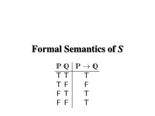
Semantics of programming languages • Basic components to describe programming languages • Syntax • Semantics • Syntax is described by a grammar • a grammar is a 4-tuple (T,N,P,s) • T: a set of symbols (terminals) • N: a set of non-terminals • s N: starting non-terminal • P: a set of productions • a production has form: a b (a, b T N) • There are many approaches to providing formal semantics to a programming language: • Operational • Denotational • Axiomatic • Algebraic
Algebraic specification of Stack and Queue QUEUE sorts: QUEUE, INT, BOOLEAN operations: new: --> QUEUE add: QUEUE x INT --> QUEUE empty: QUEUE --> BOOLEAN del: QUEUE --> QUEUE head: QUEUE --> INT U { error } Semantics empty(new()=true emtpty(add(q,i))=false del(New())=error del(add(q,i))=if (empty(q)) then new() else add(del(q),i) head(new())=error head(add(q,i))=if (empty(q)) then i else head(q) STACK sorts: STACK, INT, BOOLEAN operations: new: --> STACK push: STACK x INT --> STACK empty: STACK --> BOOLEAN pop: STACK --> STACK top: STACK --> INT U { error } Semantics empty(new()) = true empty(push(S, i)) = false pop(new()) = error pop(push(S, i)) = S top(new()) = error top(push(S,i)) = i
Axiomatic system • An axiomatic system is any set of axioms from which some or all axioms can be used in conjunction to logically derive theorems. • E.g. Euclidean geometry • Axiom: accepted unproved statement • It consists of • A grammar, i.e. a way of constructing well-formed formulae out of the symbols, such that it is possible to find a decision procedure for deciding whether a formula is a well-formed formula (wff) or not. • A set of axioms or axiom schemata: each axiom has to be a wff. • A set of inference rules. • A set of theorems. This set includes all the axioms, plus all wffs which can be derived from previously-derived theorems by means of rules of inference. • Unlike the grammar for wffs, there is no guarantee that there will be a decision procedure for deciding whether a given wff is a theorem or not.
Y N C Y N C S1 S2 S The programming language • A simple language: W ::= V := T W ::= if B then W else W W ::= while B do W W ::= W ; W • An idealized, but nonetheless quite powerful, programming language. • Remember that any program can be represented using these basic language constructs. S1 S2
Hoare Logic • We can use assertions to describe program semantics {x=0} x:=x+1 {x=1} • Hoare Logic formalizes this idea • An Hoare triple is in the following form: • {P} S {Q} where P and Q are assertions, and S is a program segment • {P} S {Q} means “if we assume that P holds before S starts executing, then Q holds at the end of the execution of S” • I.e., if we assume P before execution of S, Q is guaranteed after execution of S
Example Hoare triples • Whether the following triples are true? How can we prove? {x=0} x:=x+1 {x=1} {x+y=5} x:=x+5; y:=y-1 {x+y=9} {x+y=C} x:=x+5; y:=y-1 {x+y=C+4} where C is a place holder for any integer constant, i.e., it is equivalent to • C, {x+y=C} x:=x+5; y:=y-1 {x+y=C+4} {x>C} x:=x+1 {x>C+1} {x>C} x:=x+1 {x>C} {x=1} x:=x+1 {x=1} {x+y=C} x:=x+1; y:=y1 {x+y=C+1} incorrect incorrect
Proving properties of program segments • How can we prove that: {x=0} x:=x+1 {x=1} is correct? • We need an axiom which explains what assignment does • First, we will need more notation • We need to define the substitution operation • Let P[exp/x] denote the assertion obtained from P by replacing every appearance of x in P by the value of the expression exp • Examples (x=0)[0/x] • 0=0 (x+y=z)[0/x] 0+y=z y=z
Axiom of Assignment • Here is the axiom of assignment: {P[exp/x]} x:=exp {P} • where exp is a simple expression (no procedure calls in exp) that has no side effects (evaluating the expression does not change the state of the program) • Now, let’s try to prove {x=0} x:=x+1 {x=1} We have {x=1[x+1/x]} x:=x+1 {x=1} (by axiom of assignment) • {x+1=1} x:=x+1 {x=1} (by definition of the substitution operation) • {x=0} x:=x+1 {x=1} (by some axiom of arithmetic)
Axiom of Assignment • Another example {x0} x:=x+1 {x1} We have {x1[x+1/x]} x:=x+1 {x1} (by axiom of assignment) • {x+11} x:=x+1 {x1} (by definition of the substitution operation) • {x0} x:=x+1 {x1} (by some axiom of arithmetic)
Rules of Inference—rule of consequence • Now we know {x=0} x:=x+1 {x=1} • How can we prove {x=0} x:=x+1 {x>0} • Once we prove a Hoare triple we may want to use it to prove other Hoare triples • Here is the general rule (rule of consequence 1) • If {P}S{Q} and QQ’ then we can conclude {P}S{Q’} • Example: {x=0} x:=x+1 {x=1} and x=1x>0 • hence, we conclude {x=0} x:=x+1 {x>0}
Rules of Inference—rule of consequence • If we already proved {x0} x:=x+1 {x1}, then we should be able to conclude {x5} x:=x+1 {x1} • Here is the general rule (rule of consequence 2) • If {P}S{Q} and P’P then we can conclude {P’}S{Q} • Example • {x0} x:=x+1 {x1} and x5 x0 • hence, we conclude {x5} x:=x+1 {x1}
Rule of Sequential Composition • Program segments can be formed by sequential composition • x:=x+5; y:=y1 is sequential composition of two assignment statements x:=x+5 and y:=y-1 • x:=x+5; y:=y1; t:=0 is a sequential composition of the program segment x:=x+5; y:=y1 and the assignment statement t:=0 • How do we reason about sequences of program statements? • Here is the inference rule of sequential composition • If {P}S{Q} and {Q}T{R} then we can conclude that {P} S;T{R}
Example: Swap • prove a swap operation t:=x; x:=y; y:=t • assume that x=Ay=B holds before we start executing the swap segment. • If swap is working correctly we would like x=By=A to hold at the end of the swap (note that we did not restrict values A,B in any way) {x=Ay=B} t:=x; x:=y; y:=t {x=By=A} • apply the axiom of assignment twice {x=By=A[t/y]} y:=t {x=By=A} {x=Bt=A} y:=t {x=By=A} {x=Bt=A[y/x]} x:=y {x=Bt=A} {y=Bt=A} x:=y {x=Bt=A}
Swap example • Now since we have {y=Bt=A} x:=y {x=Bt=A} and {y=Bt=A} y:=t {x=By=A}, • using the rule of sequential composition we get: {y=Bt=A} x:=y; y:=t {x=By=A} • apply the axiom of assignment once more {y=Bt=A[x/t]} t:=x {y=Bt=A} {y=Bx=A} t:=x {y=Bt=A} • Using the rule of sequential composition once more {y=Bx=A} t:=x {y=Bt=A} and {y=Bt=A} x:=y; y:=t {x=By=A} • {y=Bx=A} t:=x; x:=y; y:=t {x=By=A}
Inference rule for conditionals • There are two inference rules for conditional statements, one for if-then and one for if-then-else statements • For if-then-else statements the rule is (rule of conditional 1) If {PB} S1 {Q} and {PB} S2 {Q} hold then we conclude that {P} if B then S1 else S2 {Q} • For if-then statements the rule is (rule of conditional 2)
Example for conditionals • Here is an example if (x >y) then max:=x else max:=y • We want to prove {True} if (x>y) then max:=x else max:=y {maxxmaxy} {maxxmaxy[x/max} max:=x {maxxmaxy} (Assignment axiom) {xxxy} max:=x {maxxmaxy} (definition of substitution) {Truexy} max:=x {maxx maxy} (some axiom of arithmetics) {xy} max:=x {maxx maxy} (some axiom of logic) {x>y} max:=x {maxx maxy} (rule of consequence 2)
Example for conditionals {maxxmaxy[maxy]} max:=y {maxxmaxy} (r.assign.) {yxyy} max:=y {maxxmaxy} (definition of subs.) {yxTrue} max:=y {max xmaxy} (some axiom of arithmetics.) {yx} max:=y {maxx maxy} (some axiom of logic) {x>y} max:=y {maxxmaxy} (some axiom of logic) So we proved that { x>y} max:=x {maxxmaxy}, and {x>y} max:=y {maxxmaxy} Then we can use the rule of conditional 1 and conclude that: {True} if (x>y) max:=x else max:=y {maxxmaxy}
Example for conditional rule 2 • Proof the following Hoare triple: {true} m:=y; if (x>y) m:=x; {mx my} We need to prove {true} m:=y; {m=y} and {m=y} if (x>y) m:=x; {mx my} To prove {m=y} if (x>y) m:=x; {mx my}, We need to show that • {m=y x>y } m:=x; {m x m y} • m=y NOT x>y ==> m x m y 2) is true. (some properties of logic)
Example for conditional rule 2 To prove : {m=y x>y } m:=x; {m x m y} {m x m y [x/m] } m:=x; {m x m y} by assignment axiom {x x x y [x/m] } m:=x; {m x m y} by simplification {x y } m:=x; {m x m y} by simplification Since m = y x>y => x y; 3) {m=y x>y } m:=x; {m x m y} by consequence rule and 3)
What about the loops? • Here is the inference rule (rule of iteration) for while loops If {PB} S {P} then we can conclude that {P} while B do S {BP } • This is what the inference rule for while loop is saying: • If you can show that every iteration of the loop preserves the property P, • and you know that the property holds before you start executing the loop, • then you can conclude that the property holds at the termination of the loop. • Also the loop condition will not hold at the termination of the loop (otherwise the loop would not terminate).
Loop invariants • Given a loop • while B do S • Any assertion P which satisfies {PB} S {P} is called a loop invariant • A loop invariant is an assertion such that, every iteration of the loop body preserves it • In terms of Hoare triples this is equivalent to {PB} S {P} • Note that rule of iteration given in the previous slide is for partial correctness • It does not guarantee that the loop will terminate
Using the rule of iteration • To prove that a property Q holds after the loop while B do S terminates, we can use the following strategy • Find a strong enough loop invariant P such that: (B P) Q • Show that P is a loop invariant: {P B} S {P} • IF we can show that P is a loop invariant, we get {P} while B do S {BP } • Since we assumed that (B P) Q, using the rule of consequence 1, we get {P} while B do S {Q}
The factorial example {true} x := 0; f := 1; while ( x != n ) do (x := x + 1; f := f * x;) {f=n!} Assume that n ≥ 0. After computing x := 0; f := 1; we have f = x!, i.e., {true} x := 0; f := 1; {f=x!} because it is true that 1 = 0! We can show that: { f = x! } x := x + 1; f := f * x; { f = x! }
The factorial again... (2) Now, P is f = x! B is x!=n B is x = n Using the inference rule for "while" loops: { f =x! } while ( x != n ) do (x := x + 1; f := f * x;) { f = x! & x = n}
The factorial again... (3) Notice that f = x! & x = nf = n! This means two things: • { true } x := 0; f := 1; { f = x! } AND { f = x! }while ( x != n ) do (x := x + 1; f := f * x;) { f = n!}
Factorial (4) In other words, the program establishes f = n! without any preconditions on the initial values of f and n, assuming that we only deal with n ≥ 0. The rule for statement composition gives us: { true } x := 0; f := 1; while ( x != n ) ( x := x + 1; f := f * x;) { f == n!} So: this program does compute the factorial of n.
Factorial(5) Our reasoning agrees with the intuition of loop invariants: we adjust some variables and make the invariant temporarily false, but we re-establish it by adjusting some other variables. { f = x! }x:= x + 1;{f = (x– 1)! } the invariant is "almost true" {f = (x– 1)! } f := f * x;{f = x! } the invariant is back to normal This reasoning is not valid for infinite loops:the terminating condition P & B is never reached, and we know nothing of the situation following the loop.
Termination • Proofs like these show only partial correctness. • Everything is fine if the loop stops. • Otherwise we don't know (but the program may be correct for most kinds of data). • A reliable proof must show that all loops in the program are finite. • We can prove termination by showing how each step brings us closer to the final condition.
Once again, the factorial… • Initially, x = 0. • Every step increases x by 1, so we go through the numbers 0, 1, 2, ... • n >= 0 must be found among these numbers. • Notice that this reasoning will not work forn < 0: the program loops.
A decreasing function • A loop terminates when the value of some function of program variables goes down to 0 during the execution of the loop. • For the factorial program, such a function could be n – x. Its value starts at n and decreases by 1 at every step.
Sum example (1) • Consider the following program segment: sum:=0; i:=1; while (i <=10) do (sum:=sum+i; i:=i+1) • We want to prove that Q sum=0 k 10k holds at the loop termination, i.e., we want to prove the Hoare triple: {true} sum:=0; i:=1; while (i <=10) do (sum:=sum+i; i:=i+1) {Q} We need to find a strong enough loop invariant P • Let’s choose P as follows: P i 11 sum=0 k<ik
Sum example (2) • To use the rule of iteration we need to show {PB} S {P} where P i 11 sum=0 k<ik S: sum:=sum+i; i:=i+1 B i 10 • Using the rule of assignment we get: {i 11 sum=0 k<ik [i+1/i]} i:=i+1 {i 11 sum=0 k<ik} • {i+1 11 sum=0 k<i+1k} i:=i+1 {i 11 sum=0 k<ik} • {i 10 sum=0 k<i+1k} i:=i+1 {i 11 sum=0 k<ik}
Sum example (3) Using the rule of assignment one more time: {i 10sum=0 k<i+1k[sum+i/sum]} sum:=sum+I{i 10sum=0 k<i+1k} {i 10 sum+i=0 k<i+1k} sum:=sum+i {i 10 sum=0 k<i+1k} • {i 10 sum=0 k<ik} sum:=sum+i {i 10 sum=0 k<i+1k} Using the rule of sequential composition we get: {i 10 sum=0 k<ik} sum:=sum+i; i:=i+1 {i 11 sum=0 k<ik}
Sum example (4) • Note that P B (i 11 sum=0 k<ik)(i 10) i 10 sum=0 k<ik P B (i 11 sum=0 k<ik) (i 10) • i 11 i 10 sum=0 k<iki = 11 sum=0 k<ik • sum=0 k<11k • Using the rule of iteration we get: {i 11 sum=0 k<ik} while (i <=10) do (sum:=sum+i; i:=i+1) {sum=0 k<11k}
Sum example (5) • To finish the proof, apply assignment axiom {i 11 sum=0 k<ik[1/i]}i:= 1 {i 11 sum=0 k<ik} • {111 sum=0 k<1k} i:= 1 {i 11 sum=0 k<ik} • { sum=0}i:= 1 {i 11 sum=0 k<ik} Another rule of assignment application {sum=0 [0/sum]} sum := 0 {sum=0} {0=0} sum := 0 {sum=0} {true} sum := 0 {sum=0}
Sum example (6) • Finally, combining the previous results with rule of sequential composition we get: • {true} • sum:=0; i:=1; while (i <=10) do (sum:=sum+i; i:=i+1) • {sum=0 k 10k}
Difficulties in Proving Programs Correct • Finding a loop invariant that is strong enough to prove the property we are interested in can be difficult • Also, note that we did not prove that the loop will terminate • To prove total correctness we also have to prove that the loop terminates • Things get more complicated when there are procedures and recursion
Difficulties in Proving Programs Correct • Hoare Logic is a formalism for reasoning about correctness about programs • Developing proof of correctness using this formalism is another issue • In general proving correctness about programs is uncomputable • For example determining that a program terminates is uncomputable • This means that there is no automatic way of generating these proofs • Still Hoare’s formalism is useful for reasoning about programs