Understanding Clustering Algorithms: Applications, Challenges, and Hierarchical Methods
This text delves into clustering algorithms, focusing on their applications and the challenges encountered with high-dimensional data. It explains fundamental concepts like the curse of dimensionality, demonstrating through examples like the SkyCat and collaborative filtering. Hierarchical clustering methods are discussed, including techniques for determining cluster nearness and representation. The differences between various distance measures, such as Euclidean and Jaccard distances, are explored, providing insight into how to effectively cluster different types of data like CDs, documents, and DNA sequences.

Understanding Clustering Algorithms: Applications, Challenges, and Hierarchical Methods
E N D
Presentation Transcript
Clustering Algorithms Applications Hierarchical Clustering k -Means Algorithms CURE Algorithm
The Problem of Clustering • Given a set of points, with a notion of distance between points, group the points into some number of clusters, so that members of a cluster are in some sense as close to each other as possible.
Example x xx x x x x x x x x x x x x x x x x x x x x x x x x x x x x x x x x x x x x x x
Problems With Clustering • Clustering in two dimensions looks easy. • Clustering small amounts of data looks easy. • And in most cases, looks are not deceiving.
The Curse of Dimensionality • Many applications involve not 2, but 10 or 10,000 dimensions. • High-dimensional spaces look different: almost all pairs of points are at about the same distance.
Example: Curse of Dimensionality • Assume random points within a bounding box, e.g., values between 0 and 1 in each dimension. • In 2 dimensions: a variety of distances between 0 and 1.41. • In 10,000 dimensions, the difference in any one dimension is distributed as a triangle.
Example – Continued • The law of large numbers applies. • Actual distance between two random points is the sqrt of the sum of squares of essentially the same set of differences.
Example High-Dimension Application: SkyCat • A catalog of 2 billion “sky objects” represents objects by their radiation in 7 dimensions (frequency bands). • Problem: cluster into similar objects, e.g., galaxies, nearby stars, quasars, etc. • Sloan Sky Survey is a newer, better version.
Example: Clustering CD’s (Collaborative Filtering) • Intuitively: music divides into categories, and customers prefer a few categories. • But what are categories really? • Represent a CD by the customers who bought it. • Similar CD’s have similar sets of customers, and vice-versa.
The Space of CD’s • Think of a space with one dimension for each customer. • Values in a dimension may be 0 or 1 only. • A CD’s point in this space is (x1, x2,…, xk), where xi = 1 iff the i th customer bought the CD. • Compare with boolean matrix: rows = customers; cols. = CD’s.
Space of CD’s – (2) • For Amazon, the dimension count is tens of millions. • An alternative: use minhashing/LSH to get Jaccard similarity between “close” CD’s. • 1 minus Jaccard similarity can serve as a (non-Euclidean) distance.
Example: Clustering Documents • Represent a document by a vector (x1, x2,…, xk), where xi = 1 iff the i th word (in some order) appears in the document. • It actually doesn’t matter if k is infinite; i.e., we don’t limit the set of words. • Documents with similar sets of words may be about the same topic.
Aside: Cosine, Jaccard, and Euclidean Distances • As with CD’s we have a choice when we think of documents as sets of words or shingles: • Sets as vectors: measure similarity by the cosine distance. • Sets as sets: measure similarity by the Jaccard distance. • Sets as points: measure similarity by Euclidean distance.
Example: DNA Sequences • Objects are sequences of {C,A,T,G}. • Distance between sequences is edit distance, the minimum number of inserts and deletes needed to turn one into the other. • Note there is a “distance,” but no convenient space in which points “live.”
Methods of Clustering • Hierarchical (Agglomerative): • Initially, each point in cluster by itself. • Repeatedly combine the two “nearest” clusters into one. • Point Assignment: • Maintain a set of clusters. • Place points into their “nearest” cluster.
Hierarchical Clustering • Two important questions: • How do you determine the “nearness” of clusters? • How do you represent a cluster of more than one point?
Hierarchical Clustering – (2) • Key problem: as you build clusters, how do you represent the location of each cluster, to tell which pair of clusters is closest? • Euclidean case: each cluster has a centroid= average of its points. • Measure intercluster distances by distances of centroids.
Example (5,3) o (1,2) o o (2,1) o (4,1) o (0,0) o (5,0) x (1.5,1.5) x (4.7,1.3) x (1,1) x (4.5,0.5)
And in the Non-Euclidean Case? • The only “locations” we can talk about are the points themselves. • I.e., there is no “average” of two points. • Approach 1: clustroid = point “closest” to other points. • Treat clustroid as if it were centroid, when computing intercluster distances.
“Closest” Point? • Possible meanings: • Smallest maximum distance to the other points. • Smallest average distance to other points. • Smallest sum of squares of distances to other points. • Etc., etc.
Example clustroid 1 2 6 4 3 clustroid 5 intercluster distance
Other Approaches to Defining “Nearness” of Clusters • Approach 2: intercluster distance = minimum of the distances between any two points, one from each cluster. • Approach 3: Pick a notion of “cohesion” of clusters, e.g., maximum distance from the clustroid. • Merge clusters whose union is most cohesive.
Cohesion • Approach 1: Use the diameter of the merged cluster = maximum distance between points in the cluster. • Approach 2: Use the average distance between points in the cluster.
Cohesion – (2) • Approach 3: Use a density-based approach: take the diameter or average distance, e.g., and divide by the number of points in the cluster. • Perhaps raise the number of points to a power first, e.g., square-root.
k – Means Algorithm(s) • Assumes Euclidean space. • Start by picking k, the number of clusters. • Initialize clusters by picking one point per cluster. • Example: pick one point at random, then k -1 other points, each as far away as possible from the previous points.
Populating Clusters • For each point, place it in the cluster whose current centroid it is nearest. • After all points are assigned, fix the centroids of the k clusters. • Optional: reassign all points to their closest centroid. • Sometimes moves points between clusters.
Reassigned points Clusters after first round Example: Assigning Clusters 2 4 x 6 3 1 8 7 5 x
Best value of k Average distance to centroid k Getting k Right • Try different k, looking at the change in the average distance to centroid, as k increases. • Average falls rapidly until right k, then changes little.
Too few; many long distances to centroid. Example: Picking k x xx x x x x x x x x x x x x x x x x x x x x x x x x x x x x x x x x x x x x x x
Just right; distances rather short. Example: Picking k x xx x x x x x x x x x x x x x x x x x x x x x x x x x x x x x x x x x x x x x x
Too many; little improvement in average distance. Example: Picking k x xx x x x x x x x x x x x x x x x x x x x x x x x x x x x x x x x x x x x x x x
BFR Algorithm • BFR (Bradley-Fayyad-Reina) is a variant of k -means designed to handle very large (disk-resident) data sets. • It assumes that clusters are normally distributed around a centroid in a Euclidean space. • Standard deviations in different dimensions may vary.
BFR – (2) • Points are read one main-memory-full at a time. • Most points from previous memory loads are summarized by simple statistics. • To begin, from the initial load we select the initial k centroids by some sensible approach.
Initialization: k -Means • Possibilities include: • Take a small random sample and cluster optimally. • Take a sample; pick a random point, and then k – 1 more points, each as far from the previously selected points as possible.
Three Classes of Points • The discard set : points close enough to a centroid to be summarized. • The compression set : groups of points that are close together but not close to any centroid. They are summarized, but not assigned to a cluster. • The retained set : isolated points.
Summarizing Sets of Points • For each cluster, the discard set is summarized by: • The number of points, N. • The vector SUM, whose ith component is the sum of the coordinates of the points in the ith dimension. • The vector SUMSQ: ith component = sum of squares of coordinates in ith dimension.
Comments • 2d + 1 values represent any number of points. • d = number of dimensions. • Averages in each dimension (centroid coordinates) can be calculated easily as SUMi/N. • SUMi = ith component of SUM.
Comments – (2) • Variance of a cluster’s discard set in dimension i can be computed by: (SUMSQi /N ) – (SUMi /N )2 • And the standard deviation is the square root of that. • The same statistics can represent any compression set.
Points in the RS Compressed sets. Their points are in the CS. A cluster. Its points are in the DS. The centroid “Galaxies” Picture
Processing a “Memory-Load” of Points • Find those points that are “sufficiently close” to a cluster centroid; add those points to that cluster and the DS. • Use any main-memory clustering algorithm to cluster the remaining points and the old RS. • Clusters go to the CS; outlying points to the RS.
Processing – (2) • Adjust statistics of the clusters to account for the new points. • Add N’s, SUM’s, SUMSQ’s. • Consider merging compressed sets in the CS. • If this is the last round, merge all compressed sets in the CS and all RS points into their nearest cluster.
A Few Details . . . • How do we decide if a point is “close enough” to a cluster that we will add the point to that cluster? • How do we decide whether two compressed sets deserve to be combined into one?
How Close is Close Enough? • We need a way to decide whether to put a new point into a cluster. • BFR suggest two ways: • TheMahalanobis distance is less than a threshold. • Low likelihood of the currently nearest centroid changing.
Mahalanobis Distance • Normalized Euclidean distance from centroid. • For point (x1,…,xk) and centroid (c1,…,ck): • Normalize in each dimension: yi = (xi -ci)/i • Take sum of the squares of the yi ’s. • Take the square root.
Mahalanobis Distance – (2) • If clusters are normally distributed in d dimensions, then after transformation, one standard deviation = d. • I.e., 70% of the points of the cluster will have a Mahalanobis distance < d. • Accept a point for a cluster if its M.D. is < some threshold, e.g. 4 standard deviations.
Should Two CS Subclusters Be Combined? • Compute the variance of the combined subcluster. • N, SUM, and SUMSQ allow us to make that calculation quickly. • Combine if the variance is below some threshold. • Many alternatives: treat dimensions differently, consider density.
The CURE Algorithm • Problem with BFR/k -means: • Assumes clusters are normally distributed in each dimension. • And axes are fixed – ellipses at an angle are not OK. • CURE: • Assumes a Euclidean distance. • Allows clusters to assume any shape.
Example: Stanford Faculty Salaries h h h e e e h e e e h e e e e h e salary h h h h h h h age
Starting CURE • Pick a random sample of points that fit in main memory. • Cluster these points hierarchically – group nearest points/clusters. • For each cluster, pick a sample of points, as dispersed as possible. • From the sample, pick representatives by moving them (say) 20% toward the centroid of the cluster.