Sorting

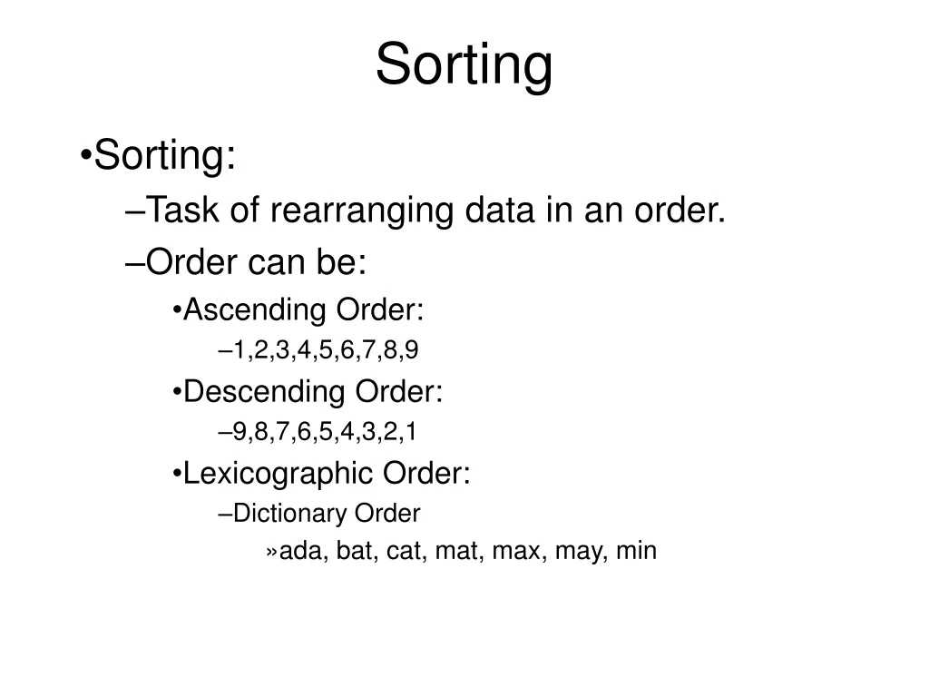
1. Sorting Sorting: Task of rearranging data in an order. Order can be: Ascending Order: 1,2,3,4,5,6,7,8,9 Descending Order: 9,8,7,6,5,4,3,2,1 Lexicographic Order: Dictionary Order ada, bat, cat, mat, max, may, min

2. Sorting Unsorted Terminologies: Sorted Stable Sort

3. Sorting Unsorted Array A Sorted Array B Not In Place Terminologies: Unsorted Array A Sorted Array A In Place Sorting

4. Sorting Terminologies: Stable Sort: A list of unsorted data may contain two or more equal data. If a sorting method maintains, The same relative position of their occurrences in the sorted list, then it is called: Stable Sort In Place Sort: Suppose a set of data to be stored is stored in an array A. If a sorting method takes place, Within the array A only, that is, without using any other extra storage space, then it is called: In Place Sorting Method Memory efficient because it does not require extra memory space.

5. Sorting Methods of Sorting: Various sorting methods are: Bubble Sort Selection Sort Insertion Sort Quick Sort Merge Sort Heap Sort

6. n = 4 Array A A[1] vs A[2] Bubble Sort A[2] vs A[3] Pass-1 A[3] vs A[4] A[1] vs A[2] A[2] vs A[3] Pass-2 A[3] vs A[4] A[1] vs A[2] A[2] vs A[3] Pass-3 A[3] vs A[4]

7. n = 4 Any optimization possible? A[1] vs A[2] Bubble Sort A[2] vs A[3] for i = 1 to n-1 do //Controls number of passes for j = 1 to n-1 do //Controls comparisons in each pass if(A[ j ] > A[ j+1 ]), then Swap(A[ j ], A[ j+1 ]) EndIf EndFor EndFor Stop Pass-1 A[3] vs A[4] A[1] vs A[2] A[2] vs A[3] Pass-2 A[3] vs A[4] A[1] vs A[2] A[2] vs A[3] Pass-3 A[3] vs A[4]

8. A[1] vs A[2] Bubble Sort A[2] vs A[3] Pass-1 A[3] vs A[4] A[1] vs A[2] A[2] vs A[3] Pass-2 A[1] vs A[2] Pass-3

9. n = 4 Bubble Sort A[1] vs A[2] Pass-1 for i = 1 to n-1 do //Controls number of passes for j = 1 to n-i do //Controls comparisons in each pass if(A[ j ] > A[ j+1 ]), then Swap(A[ j ], A[ j+1 ]) EndIf EndFor EndFor Stop A[2] vs A[3] i = 1 j = 1 to 3 A[3] vs A[4] Pass-2 A[1] vs A[2] i = 2 A[2] vs A[3] j = 1 to 2 Pass-3 A[1] vs A[2] i = 3 j = 1 to 1

10. Bubble Sort Algorithm: BubbleSort Input: Array A[1...n] where n is the number of elements. Output: Array A with all elements in ascending sorted order. Data Structure: Array A[1...n]

11. Steps: for i = 1 to n-1 do //Controls the number of passes for j = 1 to n-i do //Controls the comparisons in each pass if(A[ j ] > A[ j+1 ]), then //Logic to swap temp = A[ j ] A[ j ] = A[ j+1 ] A[ j+1 ] = temp EndIf EndFor EndFor Stop Bubble Sort

12. Tracing of Bubble Sort A[1] vs A[2] A[2] vs A[3] Pass-1 A[3] vs A[4] A[1] vs A[2] A[2] vs A[3] Pass-2 A[1] vs A[2] Pass-3

13. Tracing of Bubble Sort A[1] vs A[2] A[2] vs A[3] Pass-1 A[3] vs A[4] A[1] vs A[2] A[2] vs A[3] Pass-2 A[1] vs A[2] Pass-3

14. Tracing of Bubble Sort A[1] vs A[2] A[2] vs A[3] Pass-1 A[3] vs A[4] A[1] vs A[2] A[2] vs A[3] Pass-2 A[1] vs A[2] Pass-3

15. Exercise Tracing of Bubble Sort

16. Bubble Sort Analysis of Algorithm BubbleSort: Performance of any sorting algorithm depends on: Number of comparisons Number of movements (Swappings)

17. Analysis of algorithm BubbleSort Summary

18. min_val min_val min_loc min_loc Input Array A 40 30 50 10 20 Selection Sort Minimum element should have been at location 1. Pass-1 40 30 50 10 20 Assumption: Element at location 1 should be minimum. Is it at same location? No SWAP Minimum element should have been at location 2. Pass-2 10 30 50 40 20 Assumption: Element at location 2 should be minimum. Is it at same location? No SWAP

19. min_val min_val min_loc min_loc Selection Sort Minimum element should have been at location 3. Pass-3 10 20 50 40 30 Assumption: Element at location 3 should be minimum. Is it at same location? No SWAP Minimum element should have been at location 4. Pass-4 10 20 30 40 50 Assumption: Element at location 4 should be minimum. Is it at same location? Yes NO SWAP 10 20 30 40 50 10 20 30 40 50 Output

20. min_val min_val min_val min_val min_val min_val min_val min_val min_loc min_loc min_loc min_loc min_loc min_loc min_loc min_loc Input Array A 50 40 30 20 10 Selection Sort Minimum element should have been at location 1. Pass-1 Assumption: Element at location 1 should be minimum. 50 40 30 20 10 Is it at same location? No SWAP Minimum element should have been at location 2. Pass-2 Assumption: Element at location 2 should be minimum. 10 40 30 20 50 Is it at same location? No SWAP

21. min_val min_val min_loc min_loc 10 20 30 40 50 10 20 30 40 50 1 2 3 4 5 1 2 3 4 5 Selection Sort Minimum element should have been at location 3. Pass-3 Assumption: Element at location 3 should be minimum. 10 20 30 40 50 Is it at same location? Yes NO SWAP Minimum element should have been at location 4. Pass-4 Assumption: Element at location 4 should be minimum. 10 20 30 40 50 Is it at same location? Yes NO SWAP Output

22. To sort 5 elements, 4 passes were required. For i = 1 to n-1, do min_val = A[ i ], min_loc = i For j = i+1 to n, do If(min_val > A[ j ]), then min_val = A[ j ] min_loc = j EndIf EndFor If(i != min_loc) Swap(A[ i ], A[min_loc]) EndIf EndFor Stop Selection Sort To sort n elements, n-1 passes are required. In 1st pass, value at location 1 will be smallest. In 2nd pass, value at location 2 will be smallest. In i-th pass, value at location i will be smallest. In 1st pass, we need to do comparisons from 2nd value. In 2nd pass, we need to do comparisons from 3rd value. In ith pass, we need to start comparisons from (i+1)th value upto n.

23. Selection Sort Algorithm: SelectionSort Input: Array A[1...n] where n is the number of elements. Output: Array A with all elements in ascending sorted order. Data Structure: Array A[1...n]

24. Steps: For i = 1 to n-1, do //Controls the number of passes min_val = A[ i ], min_loc = i For j = i+1 to n, do //Controls the comparisons in each pass If(min_val > A[ j ]), then min_val = A[ j ] min_loc = j EndIf EndFor If(i != min_loc) //Swap A[ i ] and A[min_loc] temp = A[ i ] A[ i ] = A[min_loc] A[min_loc] = temp EndIf EndFor Selection Sort

25. min_val min_val min_loc min_loc Input Array A 10 20 30 40 50 Selection Sort Minimum element should have been at location 1. Pass-1 Assumption: Element at location 1 should be minimum. 10 20 30 40 50 Is it at same location? Yes NO SWAP Minimum element should have been at location 2. Pass-2 Assumption: Element at location 2 should be minimum. 10 20 30 40 50 Is it at same location? Yes NO SWAP

26. min_val min_val min_loc min_loc 10 20 30 40 50 10 20 30 40 50 1 2 3 4 5 1 2 3 4 5 Selection Sort Minimum element should have been at location 3. Pass-3 Assumption: Element at location 3 should be minimum. 10 20 30 40 50 Is it at same location? Yes NO SWAP Minimum element should have been at location 4. Pass-4 Assumption: Element at location 4 should be minimum. 10 20 30 40 50 Is it at same location? Yes NO SWAP Output

27. 40 10 10 10 10 40 10 10 10 20 20 60 60 20 20 60 60 20 50 50 40 50 50 40 50 40 50 50 10 10 40 40 40 50 40 50 20 20 60 20 60 20 60 60 60 1 1 1 1 1 1 1 1 1 2 2 2 2 2 2 2 2 2 3 3 3 3 3 3 3 3 3 4 4 4 4 4 4 4 4 4 5 5 5 5 5 5 5 5 5 Min Min Min Min Input Array A Tracing of Selection Sort Pass-1 Pass-2 Pass-3 Pass-4 No Swap

28. Tracing of Selection Sort Array A

29. Analysis of algorithm SelectionSort Summary

30. Insertion Sort Insertion Sort: Based on a method called: Bridge Player The way Bridge Player sort their hands. Picking up one card at a time, placing into its appropriate position.

31. Insertion Sort 30 50 10 20 Array A 40 40 30 50 10 20 Array B

32. B[1] = A[1] For i = 2 to n, do //Pick the element KEY = A[ i ] //Find appropriate location by comparison location = i While(location > 1) AND(KEY < B[location-1]), do location = location - 1 EndWhile //Shift elements if required j = i While( j > location ) B[ j ] = B [ j – 1 ] j = j - 1 EndWhile //Place the element B[location] = KEY EndFor Insertion Sort 1st element - Direct For all other elements 1. Pick the element 2. Find appropriate position / location. 3. Shift existing elements if required. 4. Place the element.

33. Insertion Sort Algorithm: InsertionSort Input: Array A[1...n] where n is the number of elements. Output: Array B[1...n] with elements sorted in ascending order. Data Structure: Array A[1...n] and B[1...n]

34. Steps of InsertionSort B[1] = A[1] For i = 2 to n, do //Pick the element KEY = A[ i ] //Find appropriate location by comparison location = i While(location > 1) AND (KEY < B[location-1]), do location = location - 1 EndWhile //Shift elements if required j = i While( j > location ) B[ j ] = B [ j – 1 ] j = j - 1 EndWhile //Place the element B[location] = KEY EndFor

35. Tracing of Insertion Sort 30 50 10 20 Array A 40 0 Iteration 1 3 2 4 40 Array B 30 40 30 40 50 10 30 40 50 10 20 30 40 50

36. Tracing of Insertion Sort Array A

37. Analysis of algorithm InsertionSort Summary

38. Divide & Conquer Sorting Break all the sticks into 2 parts and arrange them in order. Solution: 1) Divide: Separate the sticks from the bundle of sticks so that it could be broken. 2) Conquer (Solve / Win): Break each and every stick into 2 parts (which can be easily done) 3) Combine: Arrange all the parts in an order.

39. Quick Sort Quick Sort: To sort an array, it uses the concept of: Divide & Conquer Process: Divide a large list/array into a number of smaller lists/arrays. Sort them separately. Combine the results to get the sorted list.

40. Problem Solution P1 P2 P3 Pn Divide & Conquer Quick Sort Divide Solve . . . . . . . . Combine

41. Quick Sort left left left left right right right right loc loc loc While(A[loc] >= A[left]) While(A[loc] <= A[right]) • left = left + 1 • right = right - 1 Scan from left to right Scan from right to left X X 25 44 22 99 11 88 33

42. Quick Sort left right right right right right loc While(A[loc] >= A[left]) AND (loc > left) While(A[loc] <= A[right]) AND (loc < right) • left = left + 1 • right = right - 1 Scan from right to left Scan from left to right 44 33 99 88 22

43. Quick Sort left left left right right right loc loc loc loc Scan from left to right Scan from right to left 88 22 33 99 44 While (A[loc] <= A[right]) AND loc < right right = right - 1 While (A[loc] >= A[left]) AND loc > left left = left + 1

44. loc = left While(left < right), do //Scan from right to left While(A[loc] <= A[right]) AND (loc < right), do right = right - 1 EndWhile If(A[loc] > A[right]), then Swap(A[loc], A[right]) loc = right left = left + 1 EndIf //Scan from left to right While(A[loc] >= A[left]) AND (loc > left), do left = left + 1 EndWhile If(A[loc] < A[left]), then Swap(A[loc], A[left]) loc = left right = right - 1 EndIf EndWhile Partition Algorithm Quick Sort Initialize loc to left Scan from right to left Check as to why the scanning stopped. Scan from left to right Check as to why the scanning stopped. Repeat the scannings till left and right do not meet.

45. Quick Sort left left left right right right loc loc loc loc Scan from left to right Scan from right to left 88 22 33 99 44 While (A[loc] <= A[right]) AND loc < right right = right - 1 While (A[loc] >= A[left]) AND loc > left left = left + 1

46. Quick Sort left left left left left right right right right right loc loc loc loc loc 99 22 44 88 33 99 22

47. Quick Sort Algorithm: QuickSort Input: L: Lower Bound of Array A. U: Upper Bound of Array A. Output: Array A with elements sorted in ascending order. Data Structure: Array.

48. Quick Sort Steps: left = L, right = U if(left < right), then loc = Partition(left, right) QuickSort(left, loc – 1) QuickSort(loc + 1, right) EndIf Stop

49. Quick Sort Algorithm: Partition Input: left: Index of the leftmost element in Array A. right: Index of the rightmost element in Array A. Output: loc: Final position of the pivot element. Data Structure: Array. Remark: Element located at left is taken as the pivot element.

50. loc = left While(left < right), do //Scan from right to left While(A[loc] <= A[right]) AND (loc < right), do right = right - 1 EndWhile If(A[loc] > A[right]), then Swap(A[loc], A[right]) loc = right left = left + 1 EndIf //Scan from left to right While(A[loc] >= A[left]) AND (loc > left), do left = left + 1 EndWhile If(A[loc] < A[left]), then Swap(A[loc], A[left]) loc = left right = right - 1 EndIf EndWhile