Download
1 / 28
290 likes | 515 Vues
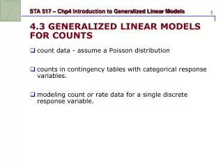
4.3 GENERALIZED LINEAR MODELS FOR COUNTS. count data - assume a Poisson distribution counts in contingency tables with categorical response variables. modeling count or rate data for a single discrete response variable. 4.3.1 Poisson Loglinear Models.

E N D
4.3 GENERALIZED LINEAR MODELS FOR COUNTS • count data - assume a Poisson distribution • counts in contingency tables with categorical response variables. • modeling count or rate data for a single discrete response variable.
4.3.1 Poisson Loglinear Models • The Poisson distribution has a positive mean µ. • Although a GLM can model a positive mean using the identity link, it is more common to model the log of the mean. • Like the linear predictor , the log mean can take any real value. • The log mean is the natural parameter for the Poisson distribution, and the log link is the canonical link for a Poisson GLM. • A Poisson loglinear GLM assumes a Poisson distribution for Y and uses the log link.
Log linear model • The Poisson loglinear model with explanatory variable X is • For this model, the mean satisfies the exponential relationship x • A 1-unit increase in x has a multiplicative impact of on µ • The mean at x+1 equals the mean at x multiplied by .
4.3.2 Horseshoe Crab Mating Example • a study of nesting horseshoe crabs. • Each female horseshoe crab had a male crab resident in her nest. • AIM: factors affecting whether the female crab had any other males, called satellites, residing nearby. • Explanatory variables are : • C - the female crab’s color, • S - spine condition, • Wt - weight, • W - carapace width. • Outcome: number of satellites (Sa) of a female crab. • For now, we only study W (carapace width)
number of satellites (Sa) = f (W) • Scatter plot – weakly linear ? (N=173) • Grouped plot: To get a clearer picture, we grouped the female crabs into width categories and calculated the sample mean number of satellites for female crabs in each category. • Figure 4.4 plots these sample means against the sample mean width for crabs in each category. • The sample means show a strong increasing trend. WHY?
SAS code data table4_3; input C S W Wt Sa@@; cards; 2 3 28.3 3.05 8 3 3 22.5 … ; procgenmoddata=table4_3; model Sa=W/dist=poisson link=identity; odsoutput ParameterEstimates=PE1; run; procgenmoddata=table4_3; model Sa=w/dist=poisson link=log; odsoutput ParameterEstimates=PE2; run;
data_NULL_; set PE1; if Parameter="Intercept"then call symput("intercp1", Estimate); if Parameter="W"thencall symput("b1", Estimate); data_NULL_; set PE2; if Parameter="Intercept"then call symput("intercp2", Estimate); if Parameter="W"thencall symput("b2", Estimate); run; data tmp; do W=22to32by0.01; mu1=&intercp1 + &b1*W; mu2=exp(&intercp2 + &b2*W); output; end; run;
Graphs procsortdata=table4_3; by W; data tmp1; merge table4_3 tmp; by W; run; symbol1i=join line=1color=green value=none; symbol2i=join line=2color=red value=none; symbol3i=none line=3value=circle; procgplotdata=tmp1; plot mu1*W mu2*W Sa*W / overlay; run;
Group data /*group data*/ data table4_3a; set table4_3; W_g=round(W-0.75)+0.75; *if W<23.25 then W_g=22.5; *if W>29.25 then W_g=30.5; run; procsql; createtable table4_3g as select W_g, count(W_g) as Num_of_Cases, sum(Sa) as Num_of_Satellites, mean(Sa) as Sa_g, var(sa) as Var_SA from table4_3a group by W_g; quit; procprint; run;
SAS output Num_of_ Num_of_ Obs W_g Cases Satellites Sa_g Var_SA 1 20.75 1 0 0.00000 . 2 21.75 1 0 0.00000 . 3 22.75 12 14 1.16667 3.0606 4 23.75 14 20 1.42857 8.8791 5 24.75 28 67 2.39286 6.5437 6 25.75 39 105 2.69231 11.3765 7 26.75 22 63 2.86364 6.8853 8 27.75 24 93 3.87500 8.8098 9 28.75 18 71 3.94444 16.8791 10 29.75 9 53 5.88889 9.8611 11 30.75 2 6 3.00000 0.0000 12 31.75 2 6 3.00000 2.0000 13 33.75 1 7 7.00000 .
Graphs data tmp2; merge table4_3g(rename=(W_g=W)) tmp; by W; run; symbol1i=join line=1color=green value=none; symbol2i=join line=2color=red value=none; symbol3i=none line=3value=circle; procgplotdata=tmp2; plot mu1*W mu2*W Sa_g*W / overlay; run;
/*fit negative binomial with identical link to count for overdispersion*/ procgenmoddata=table4_3; model Sa=W/dist=NEGBIN link=identity; odsoutput ParameterEstimates=PE3; run;
4.3.6 Poisson GLM of independence in I × J contingence tables