Pulse Code Modulation in Digital Communication Systems
Understand the basics of digital modulation with Pulse Code Modulation (PCM), covering processes like sampling and quantization. Learn about PCM transmission systems, compression laws, line codes, bandwidth of PCM signals, power spectra of line codes, and encoding schemes.

Pulse Code Modulation in Digital Communication Systems
E N D
Presentation Transcript
CHAPTER 3PULSE MODULATION Digital Communication Systems 2012 R.Sokullu
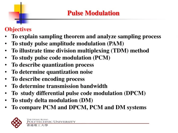
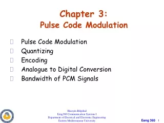
3.7 Pulse Code Modulation 3.8 Noise in PCM Systems 3.9 Time Division Multiplexing 3.10 Digital Multiplexers 3.11 Modifications of PCM Outline Digital Communication Systems 2012 R.Sokullu
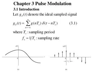
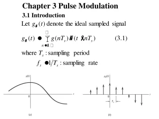
This part deals with the most basic form of digital modulation. It is based on the two main processes we have studied - the sampling process and the quantization process. Definition:Pulse Code Modulation is a technique where the message signal is represented by a sequence of coded pulses. It realizes digital representation of the signal both time-wise and amplitude-wise. 3.7 Pulse Code Modulation Digital Communication Systems 2012 R.Sokullu
PCM essentially an analog-to-digital conversion (delta modulation (DM) and differential pulse code modulation (DPCM)); special – information contained in the instantaneous sample is represented by digital words in a serial bit stream. Transmitter sampling quantization (A/DC) encoding (A/DC) Receiver regeneration decoding reconstruction Digital Communication Systems 2012 R.Sokullu
The basic elements of a PCM system. Figure 3.13 Digital Communication Systems 2012 R.Sokullu
PCM Transmission System Digital Communication Systems 2012 R.Sokullu
train of narrow rectangular pulses > 2W (sampling theorem) low-pass filter – anti-aliasing effect result = limited number of discrete values per second Sampling Digital Communication Systems 2012 R.Sokullu
Quantization • uniform law (described in sec.3.6) • non-uniform – (voice applications); step size increases in accordance with input-output amplitude separation from origin • compressor + uniform quantizer • µ-law (m and v – normalized I/O voltages) • µ-law - |m| >>1 – logarithmic; |m| << 1 – linear Digital Communication Systems 2012 R.Sokullu
Compression laws. (a) m -law. (b) A-law. Figure 3.14 Digital Communication Systems 2012 R.Sokullu
A-law Digital Communication Systems 2012 R.Sokullu
Aim – robust to noise, interference and channel impairments (see Table 3.2/204) line codes differential codes discrete set of values – appropriate signal binary codes – 1 and 0 (resistant to high noise ratio) – 256 q. levels – 8 bit code word ternary codes - 1, 0 and -1 Transmission side - Encoding Digital Communication Systems 2012 R.Sokullu
Line codes for the electrical representations of binary data. (a) Unipolar non-return-to-zero (NRZ) signaling (on-off signalling). (b) Polar NRZ signaling. (c) Unipolar return-to-zero (RZ) signaling. (d) Bipolar RZ signaling. (e) Split-phase or Manchester code. Figure 3.15 Digital Communication Systems 2012 R.Sokullu
Bandwidth of PCM Signals What is the spectrum of a PCM data waveform • For PAM – obtained as a function of the spectrum of the input analog signal, because PAM is a linear function of the signal • PCM is non-linear function of the input analog signal • Spectrum is not directly related to the spectrum of the input analog signal Bandwidth depends on: bit rate and pulse shape used to represent the data • where n is the number of bits in the PCM word, sampling frequency. For no aliasing, . (B is the analog signal bandwidth). • Dimensionality theorem gives the bounds: Digital Communication Systems 2012 R.Sokullu
Bandwidth of PCM Signals • Min bandwidth is for the case of . • Exact bandwidth depends on the type of line encoding used (unipolar NRZ, polar NRZ, bipolar RZ etc. • Next slides provide information of bandwidth and power requirements for different line encoding schemes. • For rectangular pulses first null bandwidth is: so lower bound for PCM is . Digital Communication Systems 2012 R.Sokullu
Bandwidth of PCM Signals • Finally, bandwidth for PCM signals in the case where sampling is higher than , is significantly higher than the corresponding analog signal it represents. Digital Communication Systems 2012 R.Sokullu
Power spectra of line codes: Assumptions: (a) Unipolar NRZ signal. Disadvantages – DC component; power spectra – not 0 at 0 freq. 2. Average power is normalized to unity 1. Symbols 1 and 0 are equiprobable 3. Frequency is normalized to the bit rate 1/Tb Figure 3.16a Digital Communication Systems 2012 R.Sokullu
(b) Polar NRZ signal. Disadvantages – large power near zero frequency Average power is normalized to unity Figure 3.16b Frequency is normalized to the bit rate 1/Tb Digital Communication Systems 2012 R.Sokullu
(c) Unipolar RZ signal. Advantages – presence of delta function at f=0, 1/Tb- used for syncDisadvantage – 3dB more power polar RZ for same error probability Figure 3.16c Digital Communication Systems 2012 R.Sokullu
(d) Bipolar RZ signal. Advantages – no DC component; bipolar AMI Figure 3.16d Digital Communication Systems 2012 R.Sokullu
(e) Manchester-encoded signal. Advantages – no DC; insignificant low-frequency components Figure 3.16e Digital Communication Systems 2012 R.Sokullu
encoding based on signal transitions reference signal (1) is necessary Differential Codes Figure 3.17 Digital Communication Systems 2012 R.Sokullu
PCM advantage – control effects of noise and distortion PCM signal – reconstructed by a series of regenerative repeaters along the transmission route functions: equalization – reshaping, compensates for noise and distortion timing – circuitry to provide a periodic pulse train for determining sampling instants decision making – comparison to a predetermined threshold Note: Occasional wrong decisions = bit errors Transmission Path - Regeneration Digital Communication Systems 2012 R.Sokullu
Possible problems: Noise and interference on the channel can add resulting in wrong decisions = bit errors Spacing between pulses can deviate from originally assigned = jitter Regeneration Digital Communication Systems 2012 R.Sokullu
Block diagram of regenerative repeater. Figure 3.18 Digital Communication Systems 2012 R.Sokullu
Receiver side functions regeneration regrouping into code-words decoding Decoding: generating a pulse the amplitude of which is the linear sum of all pulses in the code word, with each pulse being weighted by its place value (20, 21,…2R-1) Receiving side - Decoding Digital Communication Systems 2012 R.Sokullu
Final operation – after decoder low-pass reconstruction filter with bandwidth W (message bandwidth). If transmission path is error free the recovered signal has: no noise from channel only distortion - quantization Filtering Digital Communication Systems 2012 R.Sokullu
3.7 Pulse Code Modulation 3.8 Noise in PCM Systems 3.9 Time Division Multiplexing 3.10 Digital Multiplexers 3.11 Modifications of PCM Outline Digital Communication Systems 2012 R.Sokullu
Two major sources: channel noise quantization noise – signal dependent 3.8. Noise Considerations in PCM Systems Digital Communication Systems 2012 R.Sokullu
Channel Noise Introduces bit errors Fidelity – average probability of symbol errors (probability that the reconstructed symbol differ from the transmitted binary symbol); in BER (equal or weighted). Modeling - AWGN; reduce distance between repeaters; performance dependent on quantization noise Quantization noise –presented before; design stage Channel and Quantization Noise Digital Communication Systems 2012 R.Sokullu
BER due to AWGN depends on Eb/N0 – ratio of the transmitted signal energy per bit Eb, to the noise spectral density N0. Table 3.3 – different behavior below and above 11 dB. (compare to - 60-70 dB for high quality speech transmission with AM). No error accumulation – regeneration Error Threshold Digital Communication Systems 2012 R.Sokullu
3.7 Pulse Code Modulation 3.8 Noise in PCM Systems 3.9 Time Division Multiplexing 3.10 Digital Multiplexers 3.11 Modifications of PCM Outline Digital Communication Systems 2012 R.Sokullu
3.9. Time Division Multiplexing Figure 3.19 Digital Communication Systems 2012 R.Sokullu
1. Restricting each input by low-pass anti-aliasing filter 2. Commutator – takes sample from each input message (f > 2W); interleave samples in a frame Ts; 3. Pulse modulator – transformation for transmission over common channel 4. Pulse demodulator 5. Decommutator – synchronized with the commutator Concept Digital Communication Systems 2012 R.Sokullu
TDM - Easy to add and drop sources Pulses duration considerations time interval limited by the sampling rate (reciprocal) more users – shorter pulses – difficult to generate; highly influenced by impairments upper limit of number of independent sources Transmitter-receiver clock sync – very important – two local clocks separate code element or pulse at the end of a frame orderly procedure for detecting sync pulses – searching procedure Synchronization Digital Communication Systems 2012 R.Sokullu
24 voice channels; separate pairs of wires; regeneration every 2 km; basic to the North American Digital Switching Hierarchy Voice signal (300 – 3100 Hz) – low pass filter (cutoff frequency 3.1 kHz) – Nyquist sampling rate = 6.2 kHz – actual sampling rate 8 kHz Companding - µ-law; µ = 255; 15 piece linear segment for approximating the logarithmic characteristic; 1a, 2a, 3a … segments above x, 1b, 2b, 3b,…below x; 14 segments, each segment contains 16 uniform decision levels for segment 0 – quantizer inputs are: ±1,±3, …±31 and the outputs are 0, ±1, ….±15; for segment 1a and 1b the decision level quantizer inputs are: ±31, ±35, …±95 and the outputs are ±16, ±17,…±31 and so on for the other linear segments (up to 7a and 7b). Finally we have equally spacing on the y axis corresponding to non-equally spaced inputs on the x axis (different step for different segment); Total representation levels: 31 + 14X16 = 255 for the 15 segment companding characteristic; Example: The T1 System Digital Communication Systems 2012 R.Sokullu
Each of the 24 voice channels uses binary code with 8-bit word. first bit – 1 (positive voice input), 0 (negative voice input) bits 2 – 4 – identify particular segment last 4 bits – actual representation level (16 levels) Frames for 8 kHz, each frame occupies a period of 125 µs contains 24 X 8 =192 bit words; 1 bit for sync = 193 bits bit duration = 0.647 µs (125µs/193bits); transmission rate 1.544 Mb/s Signaling – every 6th frame, last bit; signaling rate for each channel - 8 kHz/6 = 1.333 kb/s Digital Communication Systems 2012 R.Sokullu
3.7 Pulse Code Modulation 3.8 Noise in PCM Systems 3.9 Time Division Multiplexing 3.10 Digital Multiplexers 3.11 Modifications of PCM Outline Digital Communication Systems 2012 R.Sokullu
3.10. Digital Multiplexers Same concept (TDM) used for multiplexing digital signals of different rates. Conceptual diagram of multiplexing-demultiplexing. Figure 3.20 Digital Communication Systems 2012 R.Sokullu
Multiplexing is accomplished by bit-by-bit interleaving; selector switch – sequentially scanning incoming line; at the receiving side – separation into low speed components. Types of multiplexers: relatively low data bit rate user streams are TD multiplexed over the public switched telephone network. data transmission service by telecommunication carriers; part of the national digital TDM hierarchy. Digital Communication Systems 2012 R.Sokullu
First level multiplexers – 24 64 kb/s streams (primary rate) into a DS1 (digital signal 1) stream of 1.544 Mb/s carried on the T1 system. Second level multiplexers – 4 DS1 streams into a DS2 stream at 6.312 Mb/s Third level multiplexers – 7 DS2 streams into a DS3 stream at 44.736 Mb/s Fourth level multiplexers – 6 DS3 into a DS4 stream at 274.176 Mb/s Fifth level multiplexers – 2 DS4 streams into a DS5 at 560.160 Mb/s North American Digital TDM Hierarchy Digital Communication Systems 2012 R.Sokullu
Digital transmission facilities ONLY carry bit streams without interpreting what the bits themselves mean. The two sides have common understanding of how to interpret the bits: voice, data, framing format, signaling format etc. Important Note: Digital Communication Systems 2012 R.Sokullu
1. Digital signals cannot be directly interleaved into a format that allows for their separation automatically. Common clock or perfect synchronizations is needed. The multiplexed signal must include some form of framing so the individual streams can be identified at the source. The multiplexer should be able to handle small variations in bit rates – bit stuffing. Problems: Digital Communication Systems 2012 R.Sokullu
To make the outgoing rate of the multiplexer a little bit higher than the sum of the max expected input rates. Each input is fed into an elastic store at the multiplexer (reading can be done at different rate). Identify stuffed bits – example AT&T M12 Multiplexer. Bit stuffing Digital Communication Systems 2012 R.Sokullu
Designed to combine 4 DS1 into one DS2 bit stream Each frame contains total of 24 control bits, separated by sequences of 48 data bits 4 frames, transmitted one after the other 12 bits from each input bit-by-bit interleaved, 48 bits Four types of control bits – F,M and C inserted by multiplexer – total of 24 control bits Example: signal format of the AT&T M12 Multiplexer Digital Communication Systems 2012 R.Sokullu
Signal format of AT&T M12 multiplexer Figure 3.21 Digital Communication Systems 2012 R.Sokullu
F – 2 per subframe; main framing pulses (01010101) M – 1 pr subframe; secondary framing, identifying the subframes (0111) C – 3 per subframe; stuffing indicators; indexes denote input channel; first subframe has 3 C bits, indicating stuffing in first DS1 stream; value 1 of all three indicates stuffed bits; value 0 – no stuffed bits; majority logic decoding if there is stuffing position of stuffing is – first bit after F1 Control bits Digital Communication Systems 2012 R.Sokullu
1. Searches for main framing sequence – 01010101 in F bits 2. Establishes the identity of the four DS1 streams and position of M and C bits 3. From the position of the M bits the correct position of the C bits is verified 4. Streams properly demultiplexed and destuffed. Safeguards: Double checking F and M bits for framing. Single error correction capability built into the C-control bits ensures that the 4 DS1 streams are properly destuffed Receiver Digital Communication Systems 2012 R.Sokullu
3.7 Pulse Code Modulation 3.8 Noise in PCM Systems 3.9 Time Division Multiplexing 3.10 Digital Multiplexers 3.11 Modifications of PCM Outline Digital Communication Systems 2012 R.Sokullu
Advantages: 1. Robustness to channel noise and interference. 2. Signal regeneration possibilities along the path. 3. Efficient trade-off between increased bandwidth and improved SNR (exponential law) 4. Integration of different base-band signals. 5. Comparative easy of add and drop sources. 6. Secure communication (special modulation, encryption). 3.11. Virtues, Limitations and Modifications of PCM Digital Communication Systems 2012 R.Sokullu