Transitional Trends in Pulse Modulation for Digital Communication Systems
This chapter bridges analog and digital modulation techniques by introducing pulse modulation, where parameters of a pulse train vary according to the message signal. Explore the concepts of introduction, sampling, amplitude modulation, bandwidth-noise trade-off, and more in digital communication systems.

Transitional Trends in Pulse Modulation for Digital Communication Systems
E N D
Presentation Transcript
CHAPTER 3PULSE MODULATION Digital Communication Systems 2012 R.Sokullu
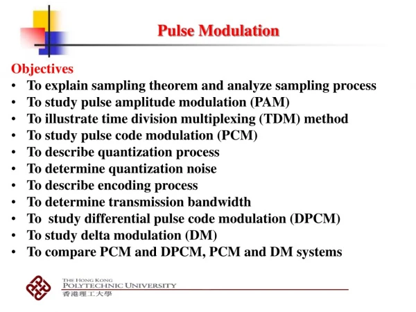
3.1 Introduction 3.2 Sampling Process 3.3 Pulse Amplitude Modulation 3.4 Other Forms of Pulse Modulation 3.5 Bandwidth-Noise Trade-off 3.6 The Quantization Process Outline Digital Communication Systems 2012 R.Sokullu
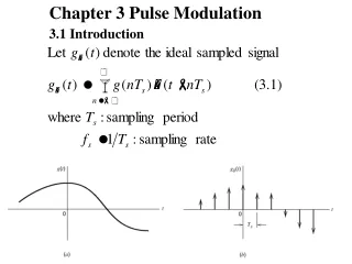
This chapter is a transitional chapter between analog and digital modulation techniques. In CW modulation, as we have studied in chapter 2, one parameter of the sinusoidal carrierwave is continuously varied in accordance with a given message signal. In the case of pulse modulation we have a pulse train and some parameter of the pulse train is varied in accordance with the message signal. 3.1 Introduction Digital Communication Systems 2012 R.Sokullu
In the first part of Communication Systems we studied transmission techniques of analog waveforms (analog sources) over analog signals (lines). Why is modulation necessary? What types of modulation did we study? When we studied a specific modulation type what were the specific subjects we discussed? CommSystems 1 – Analog Communication Techniques Digital Communication Systems 2012 R.Sokullu
In the second part we have two major topics analog waveforms (analog sources) transmission using baseband signals digital waveforms (digital sources) transmission using band-pass signals CommSystems 2 – Digital Communication Techniques Digital Communication Systems 2012 R.Sokullu
Digital approximation of analog signals can be made as precise as required Low cost of digital circuits Flexibility of digital approach – possibility of combining analog and digital sources for transmission over digital lines Increased efficiency – source coding/channel coding separation Why digital? Digital Communication Systems 2012 R.Sokullu
To study digital communication systems and their conceptual basis in information theory To study how analog waveforms can be converted to digital signals (PCM) Compute spectrum of digital signals Examine effects of filtering – how does filtering affect the ability to recover digital information at the receiver. filtering produces ISI in the recovered signal Study how to multiplex data from several digital bit streams into one high speed digital stream for transmission over a digital system (TDM) Goals of this course: Digital Communication Systems 2012 R.Sokullu
Digital transmission –1960s Real application – after 1970s developments in solid state electronics, micro-electronics, large scale integration all common information sources are inherently analog Historical steps Sampled analog sources transmitted using analog pulse modulation (PAM, PPM) Samples are quantized to discrete levels (PCM, DM) Conversion from analog and transmission were implemented as a single step Today Layered approach – different steps are distinguished and separately optimized (source coding and channel coding) Motivation and Development Digital Communication Systems 2012 R.Sokullu
We distinguish between: analog pulse modulation a periodic pulse train is used as a carrier wave; a parameter of that train (amplitude, duration, position) is varied in a continuous manner in accordance with the corresponding sample value of the message signal; information is transmitted basically in analog form, but at discrete times. digital pulse modulation message represented in a discrete way in both time and amplitude; sequence of coded pulses is transmitted. Digital Communication Systems 2012 R.Sokullu
Digital Communication Systems 2012 R.Sokullu
Problem of coding: efficient representation of source signals (speech waveforms, image waveforms, text files) as a sequence of bits for transmission over a digital network Paired problem of source decoding – conversion of received bit sequence (possibly corrupted) into a more-or-less faithful replica of the original Source Coding Digital Communication Systems 2012 R.Sokullu
Problem of the efficient transmission of a sequence of bits through a lower layer channel 4 KHz telephone channel, wireless channel Recovery at the channel output in the remote receiver despite distortions Channel Coding Digital Communication Systems 2012 R.Sokullu
Basic theorem of information theory: If a source signal can be communicated through a given point-to-point channel within some level of distortion (by any means) then the separate source and channel coding can also be designed to stay within the same limits of distortion. WHY then…(delay, complexity…) Pros and cons? Does it always hold true? Why separate source and channel coding? Digital Communication Systems 2012 R.Sokullu
Channel coding can help reduce the error probability without reducing the data rate Date rate depends on the channel itself – channel capacity Channel bandwidth W, input power P, noise power then the channel capacity in bits is: Shannon and the Channel Coding Theorem Digital Communication Systems 2012 R.Sokullu
Interface between source coding/channel coding – issues continuity, rate etc. continuous sources packet sources complex combinations Here: min number of bits from source and max transmission speed over channel source coder rate = channel encoder rate (source-channel coding theorem) Digital Interface protocols discussed in details in Data Communications course Digital Communication Systems 2012 R.Sokullu
3.1 Introduction 3.2 Sampling Process 3.3 Pulse Amplitude Modulation 3.4 Other Forms of Pulse Modulation 3.5 Bandwidth-Noise Trade-off 3.6 The Quantization Process Outline Digital Communication Systems 2012 R.Sokullu
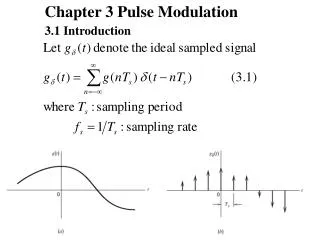
Sampling converts an analog signal into a corresponding sequence of samples that are uniformly distributed in time. Proper selection of the sampling rate is very important because it determines how uniquely the samples would represent the original signal. It is determined according to the so called sampling theorem. 3.2 Sampling Process Digital Communication Systems 2012 R.Sokullu
The model: we consider an arbitrary signal g(t) with finite energy, specified for all time we sample the signal instantaneously and at an uniform rate, once every Ts seconds we obtain an infinite sequence of samples spaced Ts seconds apart; they are denoted by [g(nTs)], where n can take all possible integer values Ts is referred to as the sampling period, and fs=1/Ts is the sampling rate. let gδ(t) denote the signal obtained by individually weighting the elements of a periodic sequence of delta functions spaced Ts seconds apart by the numbers [g(nTs)]. Digital Communication Systems 2012 R.Sokullu
The sampling process. (a) Analog signal. (b) Instantaneously sampled version of the analog signal. Figure 3.1 Digital Communication Systems 2012 R.Sokullu
For the signal gδ(t), called the ideal sampled signal, we have the following expression : • As the idealized delta function has unit area, the multiplication factor g(nTs) can be considered as “mass” assigned to it (samples are “weighted”); • A delta function weighted in this manner is approximated by a rectangular pulse of duration Δt and amplitude g(nTs)/Δt. Digital Communication Systems 2012 R.Sokullu
Knowing that the uniform sampling of a continuous-time signal of finite energy results into a periodic spectrum with a period equal to the sampling rate using the FT gδ(t) can be expressed as: • So if we take FT on both sides of (3.1) we get: discrete time Fourier transform Digital Communication Systems 2012 R.Sokullu
The relations derived up to here apply to any continuous time signal g(t) of finite energy and infinite duration. If the signal g(t) is strictly band-limited, with no components above W Hz, then the FT G(f) of g(t) will be zero for |f| ≥ W. Digital Communication Systems 2012 R.Sokullu
(a) Spectrum of a strictly band-limited signal g(t). (b) Spectrum of the sampled version of g(t) for a sampling period Ts = 1/2 W. Figure 3.2 Digital Communication Systems 2012 R.Sokullu
For a sampling period Ts=1/2 W after substitution in3.3we get the following expression: • and using 3.2 for the FT of gδ(t)we can also write: m=0 Digital Communication Systems 2012 R.Sokullu
and for the conditions specified about f we get: • and when we substitute (3.4) and (3.6) we get: Digital Communication Systems 2012 R.Sokullu
1. If the sample values g(n/2W) of an analog signal g(t) are specified for all n, then the FT G(f) of the signal is uniquely determined by using the discrete-time FT of equation (3.7). 2. Because g(t) is related to G(f) by the inverse FT, the signal g(t) is itself uniquely determined by the sample values g(n/2W) for -∞ < n <+∞. Conclusion: Digital Communication Systems 2012 R.Sokullu
Second part: reconstructing the signal from the samples • We substitute equation (3.7) in the inverse FT formula and after some reorganizing we get: • which after integration ends to be: Digital Communication Systems 2012 R.Sokullu
This is an interpolation formula for reconstructing the original signal g(t) from a sequence of sample values [g(n/2W)]. The sinc function sinc(2Wt) is playing the role of interpolation function. Each sample is multiplied by a suitably delayed version of the interpolation function and all the resulting waveforms are summed up to obtain g(t). Digital Communication Systems 2012 R.Sokullu
1. A band-limited signal of finite energy, which has no frequency components higher than W Hz, is completely described by specifying the values of the signal at instants of time separated by 1/2W (means that sampling has to be done at a rate twice the highest frequency of the original signal). 2. A band-limited signal of finite energy, which has no frequency components higher than W Hz, may be completely recovered from a knowledge of its samples taken at the rate of 2W samples per second. Sampling Theorem Digital Communication Systems 2012 R.Sokullu
The sampling rate of 2W for a signal of bandwidth W Hz, is called the Nyquist rate; Its reciprocal 1/2W (seconds) is called the Nyquist interval; Note: Digital Communication Systems 2012 R.Sokullu
The derivations of the sampling theorem so far were based on the assumption that the signal g(t) is strictly band limited. Practically – not strictly band-limited; the result is under sampling so some aliasing is produced by the sampling process. Aliasing is the phenomenon of a high-frequency component in the spectrum of the signal taking on the identity of a lower frequency in the spectrum of its sampled version. Digital Communication Systems 2012 R.Sokullu
(a) Spectrum of a signal. (b) Spectrum of an undersampled version of the signal exhibiting the aliasing phenomenon. Figure 3.3 Digital Communication Systems 2012 R.Sokullu
Practically there are two possible engineering solutions: prior to sampling, a low-pass anti-aliasing filter is used to attenuate the high-frequency components that are not essential to the information baring signal. the filtered signal is sampled at a rate slightly higher than the Nyquist rate. Note: This also makes the design of the reconstructing filter easier. Digital Communication Systems 2012 R.Sokullu
Anti-alias filtered spectrum of an information-bearing signal. (b) Spectrum of instantaneously sampled version of the signal, assuming the use of a sampling rate greater than the Nyquist rate. (c) Magnitude response of reconstruction filter. Figure 3.4 Digital Communication Systems 2012 R.Sokullu
The reconstruction filter is low-pass, pass-band –W to +W. The transition band of the filter is fs- W where fs is the sampling rate. Digital Communication Systems 2012 R.Sokullu
3.1 Introduction 3.2 Sampling Process 3.3 Pulse Amplitude Modulation 3.4 Other Forms of Pulse Modulation 3.5 Bandwidth-Noise Trade-off 3.6 The Quantization Process Outline Digital Communication Systems 2012 R.Sokullu
Definition: In Pulse Amplitude Modulation (PAM) the amplitudes of regularly spaced pulses are varied in accordance with the corresponding sample values of the continuous message signal; Note: Pulses can be rectangular or some other form. 3.3 Pulse Amplitude Modulation Digital Communication Systems 2012 R.Sokullu
Flat-top samples, representing an analog signal. Figure 3.5 Digital Communication Systems 2012 R.Sokullu
Steps in realizing PAM: Instantaneous sampling of the message signal every Ts seconds, with sampling rate fs chosen according to the sampling theorem. Lengthening the duration of each sample to obtain a constant value of T (duration of pulses). These two are known as “sample and hold”. Question is: how long should be the pulses (T)? PAM Digital Communication Systems 2012 R.Sokullu
Assume: • s(t) sequence of flat-top pulses generated as described. • where Ts is the sampling period, m(nTs) is the sample value at time t=nTs • standard rectangular pulse is represented by: • by definition the instantaneously sampled version of m(t) is: time-shifted delta function Digital Communication Systems 2012 R.Sokullu
after convolution and applying the sifting property of the delta function we get: Digital Communication Systems 2012 R.Sokullu
The result in the previous slide means that (compare 3.10 and 3.14) the PAM signal s(t) is mathematically represented by 3.15: Digital Communication Systems 2012 R.Sokullu
After taking FT on both sides we get: • Using formula 3.2 for the relation between Mδ(f) and M(f), the FT of the original message m(t) we can write: • Finally, after substitution of 3.16 into 3.17 we get • which represents the FT of the PAM signal s(t). Digital Communication Systems 2012 R.Sokullu
Second part: recovery procedure • assume that the message is limited to bandwidth W and the sampling rate is fs which is higher than the Nyquist rate. • pass s(t) through a low-pass filter whose frequency response is defined in 3.4c • the result, according to 3.18 is M(f)H(f), which is equal to passing the original signal m(t) through another low-pass filter with frequency response H(f). Fig. 3.4 Digital Communication Systems 2012 R.Sokullu
To determine H(f) we use the FT of a rectangular pulse, plotted on fig. 3.6a and 3.6b: • By using flat-top samples to generate a PAM signal we introduce amplitude distortion and delay of T/2 • This distortion is known as the aperture effect. • This distortion is corrected by the use of an equalizer after the low-pass filters to compensate for the aperture effect. The magnitude response of the equalizer is ideally: Digital Communication Systems 2012 R.Sokullu
Rectangular pulse h(t). (b) Spectrum H(f), made up of the magnitude |H(f)|, and phase arg[H(f)] Figure 3.6 Digital Communication Systems 2012 R.Sokullu
1. Transmission of a PAM signal imposes strict requirements on the magnitude and phase responses of the channel, because of the relatively short duration of the transmitted pulses. 2. Noise performance can never be better than a base-band signal transmission. 3. PAM is used only for time division multiplexing. Later on for long distance transmission another subsequent pulse modulation is used. Conclusion on PAM: Digital Communication Systems 2012 R.Sokullu
3.1 Introduction 3.2 Sampling Process 3.3 Pulse Amplitude Modulation 3.4 Other Forms of Pulse Modulation 3.5 Bandwidth-Noise Trade-off 3.6 The Quantization Process Outline Digital Communication Systems 2012 R.Sokullu
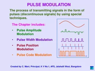
Rough comparison between CW modulation and pulse modulation shows that latter inherently needs more bandwidth. This bandwidth can be used for improving noise performance. Such additional improvement is achieved by representing the sample values of the message signal by some other parameter of the pulse (different than amplitude): pulse duration (width) modulation (PDM) – samples are used to vary the duration of the individual pulses. pulse-position modulation (PPM) – position of the pulse, relative to its un-modulated time of occurrence in accordance with the message signal. 3.4 Other Forms of Pulse Modulation Digital Communication Systems 2012 R.Sokullu
Illustrating two different forms of pulse-time modulation for the case of a sinusoidal modulating wave. (a) Modulating wave. (b) Pulse carrier. (c) PDM wave. (d) PPM wave. Figure 3.8 Digital Communication Systems 2012 R.Sokullu