Chow-Vizsla Hybrid Disposition Prediction Study
Explore using appearance to predict disposition in Chow-Vizsla hybrids. Analyze data and fit linear equations to make predictions.

Chow-Vizsla Hybrid Disposition Prediction Study
E N D
Presentation Transcript
Curve Fitting Introduction to Mathematical Modeling
Source of Example The chow/vizsla example is from “Lessons for A First Course in System Dynamics Modeling v1.0” by Diana M. Fisher. Summer Creek Press, 1998. Introduction to Mathematical Modeling
Procedure • Given paired data points (xi,yi). • Produce a scatterplot of the paired data points. • Fit a linear equationY = aX+band its graph (curve) to the data. • Evaluate the fit. • Analyze the result. Introduction to Mathematical Modeling
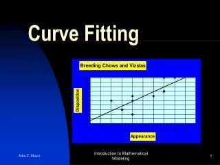
Research Question • Can the appearance of a chow-vizsla hybrid be used to predict its disposition? • Dogs are rated based upon their chow-like and vizsla-like characteristics. • Scale 0 (most like vizsla) to 10 (most like chow). Introduction to Mathematical Modeling
Table of Data Introduction to Mathematical Modeling
Scatterplot of Data Introduction to Mathematical Modeling
Plotting the Means (x,y)=(5,5.82) Introduction to Mathematical Modeling
Adding a Trendline e2 e1 e3 Introduction to Mathematical Modeling
Least Squares Fit • Minimize the error sum of squares Q = (ei)2 • The smaller Q, the closer the correlation coefficient R2 is to 1. • A perfect fit (all points on the line) has R2=1. Introduction to Mathematical Modeling
Trendline and Equation Introduction to Mathematical Modeling
No Correlation • This graph shows essentially no correlation between the variables X and Y. Introduction to Mathematical Modeling
High Correlation • This graph shows a high degree of correlation between X and Y. Introduction to Mathematical Modeling
Outliers • Outliers affect the degree of correlation. • Outliers affect the fitted curve. Introduction to Mathematical Modeling

