Download
1 / 30
300 likes | 331 Vues
Presentation on HYSPLIT modeling in Phase II of the EMEP Mercury Modeling Intercomparison Study. Discussed impacts, source-receptor relationships, chemical equilibrium, and assumptions affecting mercury deposition.

E N D
HYSPLIT Modelingin Phase II of theEMEP Mercury Modeling Intercomparison Study Dr. Mark Cohen Physical Scientist NOAA Air Resources Laboratory Silver Spring, Maryland Presentation at the Expert Meeting on Mercury Model Comparison MSC-East, Moscow, Russia April 15-16, 2003
Is the source’s impact on any given receptor proportional to its emissions? (for the same emissions speciation) RECEPTOR Source ? = Impact of 1 gram/hr source Impact of 5 gram/hr source 5 x
Impact of source 4 estimated from weighted average of impacts of nearby explicitly modeled sources 4 Spatial interpolation Impacts from Sources 1-3 are Explicitly Modeled 1 RECEPTOR 2 3
Comparison of interpolated transfer coefficients to the Great Lakes with explicitly modeled transfer coefficients for 2378 TCDD and OCDD
Transfer Coefficients for Hg are strongly influenced by the “type” of Hg emitted [Hg(II) has much greaterlocal impacts than Hg(0)]
“Chemical Interpolation” RECEPTOR Source 0.3 x Impact of Source Emitting Pure Hg(0) Impact of Source Emitting 30% Hg(0) 50% Hg(II) 20% Hg(p) + = 0.5 x Impact of Source Emitting Pure Hg(II) + 0.2 x Impact of Source Emitting Pure Hg(p)
Intersection of plumes from the two sources Source 1 Source 2 Do the emissions from one source affect the fate and transport of emissions from another source? If interaction is important, then sources not independent, and Eulerian approach is needed
Why might the atmospheric fate of mercury emissions be essentially linearly independent? • Hg is present at extremely trace levels in the atmosphere • Hg won’t affect meteorology • (can simulate meteorology independently, • and provide results to drive model) • Most species that complex or react with Hg are generally present at much higher concentrations than Hg • Other species (e.g. OH) generally react with many other compounds than Hg, so while present in trace quantities, their concentrations cannot be strongly influenced by Hg • Wet and dry deposition processes are generally 1st order with respect to Hg • The current “consensus” chemical mechanism (equilibrium + reactions) does not contain any equations that are not 1st order in Hg
Chemical Equilibrium and Reaction Scheme for Atmospheric Mercury
Correlation Coefficient = - 0.03 But daily avg conc not too far off…
In the first version of the HYSPLIT-Hg model used in this intercomparison, Hg(p) was assumed to be completely converted to dissolved Hg(II) whenever a particle becomes a droplet (e.g., above approximately 80% relative humidity); and dissolved Hg(II) assumed to become Hg(p) whenever the droplet dries out • Hg(p) and Hg(II) were thus somewhat “equivalent” in the model • With this assumption, the model tended to underpredict Hg(p) and overpredict Hg(II), suggesting that the assumption of complete conversion was not valid. • However, it was encouraging to note that the model was getting approximately the right answer for the sum of the two forms of mercury (Hg(p) + Hg(II), representing the total pool of oxidized Hg in the atmosphere [see the following graphs]
As a result of this observation, the model was re-run with the assumption that Hg(p) was not soluble. With this assumption, the results for Hg(p) and RGM were dramatically better. [These new results are what have been shown in this presentation, except for the immediately preceding RGM+Hg(p) graphs] The affect of changing this assumption had a negligible impact on Hg(0), as might be expected, given the generally very low concentrations of Hg(II) and Hg(p) relative to Hg(0).
Some Concluding Notes The version of HYSPLIT-Hg used for these calculations represented a very early stage of development of the model. The model has been changed significantly since these runs… (hopefully improved!) Methodology assumes linear independence of sources; potential advantage that detailed source-receptor relationships can be estimated Hg(p) solubility? It may be useful to reconsider some of the model evaluation metrics