Data Warehouse - Introduction

1. Data Warehouse - Introduction • Data warehousing provides architectures and tools for business executives or managers to systematically organize , understand and use their data to make strategic decisions. • Many industries spent lot of amount in building DWH. • DWH is a latest marketing weapon.(it is a way of retain users) Definition:- “A data warehouse is asubject-oriented, integrated, time-variant, and nonvolatilecollection of data which is used for decision-making process.”— W. H. Inmon G.Karuna, GRIET

2. Data Warehouse - Introduction • Subject oriented :- • Organized around major subjects, such as customer, product, sales, item etc. • Focusing on the modeling and analysis of data for decision makers, not on daily operations or transaction processing. • Provide a simple and concise view around particular subject. • Integrated:- • Constructed by integrating multiple, heterogeneous data sources like relational databases, flat files, on-line transaction records and put in a consistent format. G.Karuna, GRIET

3. Data Warehouse - Introduction • Time-variant:- • The Data are stored to provide information from a historical perspective. • Implicitly or explicitly the key structure in DWH contains an element of time. • Non-volatile :- • DWH is always a physically separate store of data, transformed from application data found in operational environment. • Operational update of data does not occur in the data warehouse environment. Only we can extract data, but we do not modify. G.Karuna, GRIET

4. Data Warehouse vs. Operational DBMS • OLTP Systems:- • Major task – to perform on line transaction, Query processing • Day-to-day operations: purchasing, inventory, banking, manufacturing, payroll, registration, accounting, etc. • OLAP Systems:- • Major task – to perform data analysis & decision making for knowledge workers. • Data organized in different formats. • Distinct features (OLTP vs. OLAP):- • User and system orientation: customer vs. market • Data contents: current, detailed vs. historical, consolidated • Database design: ER + application vs. star + subject • Access patterns: update vs. read-only but complex queries G.Karuna, GRIET

5. OLTP vs. OLAP G.Karuna, GRIET

6. Why Separate Data Warehouse? • To promote High performance for both systems. • DBMS — tuned for OLTP: access methods, indexing, searching, concurrency control, recovery • Warehouse—tuned for OLAP: complex OLAP queries, computations, multidimensional view, consolidation. • If we use OLAP in operational DB – it degrades performance • OLTP supports concurrency & recovery - if these applied on DWH it reduces the throughput. • DSS require historical data but operational DB do not maintain. • DSS requires consolidation of data from heterogeneous sources but operational contains only raw data. • Two systems support quite different functionalities. Thus we need separate DWH. • Many vendors trying to optimize OLTP db, so that they support OLAP in future. G.Karuna, GRIET

7. From Tables and Spreadsheets to Data Cubes • A data warehouse & OLAP tools are based on a multidimensional data model which views data in the form of a data cube. • A data cube, allows data to be modeled and viewed in multiple dimensions. i.e data cube is defined by dimensions and facts. • Dimension tables, such as item (item_name, brand, type), or time(day, week, month, quarter, year) • Fact table contains measures (such as dollars_sold) and keys to each of the related dimension tables. • The physical structure of DWH is a data cube. • Data cube provides multidimensional view and allows pre-computation and fast accessing of consolidated data. G.Karuna, GRIET

8. From Tables and Spreadsheets to Data Cubes Ex:- All electronics company may create DWH to keep records of sales with respect to 4 dimensions item, time, supplier, location. • Each dimension may associated with a table – Dimension table. Ex:- item is dimension (item-name, type, ….) • A data cube organized around central theme – Fact table. Ex:- sales (dollas_sold, units_sold) • In DWH, data cube is n-dimensional and it is combination of dimensions and fact tables. • Before multi-dimensional model we start with 2D cube. G.Karuna, GRIET

9. From Tables and Spreadsheets to Data Cubes • In data warehousing literature, a data cube is also referred as a cuboid. • Given set of dimensions we can generate a cubiod for each of possible subsets. The result would form a lattice of cuboids which shows the data at different levels of summarization (or) group by. • The resultant lattice of cuboids is called as n-Dimensional Data cube. • The cuboid that holds lowest level summarization is called a base cuboid. The top most is 0-D cuboid, which holds the highest-level of summarization, is called the apex cuboid. The lattice of cuboids forms a data cube. G.Karuna, GRIET

10. all 0-D(apex) cuboid time item location supplier 1-D cuboids time,location item,location location,supplier 2-D cuboids time,supplier item,supplier time,location,supplier 3-D cuboids item,location,supplier time,item,supplier 4-D(base) cuboid Cube: A Lattice of Cuboids time,item time,item,location time, item, location, supplier G.Karuna, GRIET

11. Conceptual Modeling of Data Warehouses • Modeling data warehouses: dimensions & measures • Star schema: • Popular and commonly used model. • DWH contains a large central table containing of the bulk of data with no redundancy called as fact table. • A set of small attendant tables one for each dimension called as dimension tables (de-normalized tables). • This schema looks like a star burst with central fact and surrounding with dimension tables. • The fact table contains key attributes of Dimensions. G.Karuna, GRIET

12. item time item_key item_name brand type supplier_type time_key day day_of_the_week month quarter year location branch location_key street city state_or_province country branch_key branch_name branch_type Example of Star Schema Sales Fact Table time_key item_key branch_key location_key units_sold dollars_sold avg_sales Measures G.Karuna, GRIET

13. Conceptual Modeling of Data Warehouses • Snowflake schema: • A refinement of star schema. • In this some dimension tables are normalized into a set of smaller dimension tables further. i.e. splitting the data into additional tables. • Single fact table with multiple normalized dimension tables forming a shape similar to snowflake. • To reduce redundancy, this model kept as normalized form. G.Karuna, GRIET

14. supplier item time item_key item_name brand type supplier_key supplier_key supplier_type time_key day day_of_the_week month quarter year location city branch location_key street city_key city_key city state_or_province country branch_key branch_name branch_type Example of Snowflake Schema Sales Fact Table time_key item_key branch_key location_key units_sold dollars_sold avg_sales Measures G.Karuna, GRIET

15. Conceptual Modeling of Data Warehouses • Fact constellation schema: • Sophisticated applications may require multiple fact tables to share multiple dimension tables. • Multiple fact tables with multiple dimension tables, viewed as a collection of stars, therefore called galaxy schema or fact constellation. G.Karuna, GRIET

16. item time item_key item_name brand type supplier_type time_key day day_of_the_week month quarter year location location_key street city province_or_state country shipper branch shipper_key shipper_name location_key shipper_type branch_key branch_name branch_type Example of Fact Constellation Shipping Fact Table time_key Sales Fact Table item_key time_key shipper_key item_key from_location branch_key to_location location_key dollars_cost units_sold units_shipped dollars_sold avg_sales Measures G.Karuna, GRIET

17. Cube Definition Syntax in DMQL • DMQL used to specify tasks for DWH like SQL for DBMS. • DWH can be defined using 2 language primitives. Cube Definition (Fact Table) define cube <cube_name> [<dimension_list>]: <measure_list> Dimension Definition (Dimension Table) define dimension <dimension_name> as (<attribute_or_subdimension_list>) G.Karuna, GRIET

18. Defining Star Schema in DMQL define cube sales_star [time, item, branch, location]: dollars_sold = sum(sales_in_dollars), avg_sales = avg(sales_in_dollars), units_sold = count(*) define dimension time as (time_key, day, day_of_week, month, quarter, year) define dimension item as (item_key, item_name, brand, type, supplier_type) define dimension branch as (branch_key, branch_name, branch_type) define dimension location as (location_key, street, city, province_or_state, country) G.Karuna, GRIET

19. Defining Snowflake Schema in DMQL define cube sales_snowflake [time, item, branch, location]: dollars_sold = sum(sales_in_dollars), avg_sales = avg(sales_in_dollars), units_sold = count(*) define dimension time as (time_key, day, day_of_week, month, quarter, year) define dimension item as (item_key, item_name, brand, type, supplier(supplier_key, supplier_type)) define dimension branch as (branch_key, branch_name, branch_type) define dimension location as (location_key, street, city(city_key, province_or_state, country)) G.Karuna, GRIET

20. Defining Fact Constellation in DMQL define cube sales [time, item, branch, location]: dollars_sold = sum(sales_in_dollars), avg_sales = avg(sales_in_dollars), units_sold = count(*) define dimension time as (time_key, day, day_of_week, month, quarter, year) define dimension item as (item_key, item_name, brand, type, supplier_type) define dimension branch as (branch_key, branch_name, branch_type) define dimension location as (location_key, street, city, province_or_state, country) define cube shipping [time, item, shipper, from_location, to_location]: dollar_cost = sum(cost_in_dollars), unit_shipped = count(*) define dimension time as time in cube sales define dimension item as item in cube sales define dimension shipper as (shipper_key, shipper_name, location as location in cube sales, shipper_type) define dimension from_location as location in cube sales define dimension to_location as location in cube sales G.Karuna, GRIET

21. Measures of Data Cube: Three Categories • A data cube measures - kind of aggregate function used (i) Distributive: if the result derived by applying the function to n aggregate values is the same as that derived by applying the function on all the data without partitioning E.g., count(), sum(), min(), max() (ii) Algebraic:if it can be computed by an algebraic function with M arguments (where M is a bounded integer), each of which is obtained by applying a distributive aggregate function E.g.,avg() (iii) Holistic: if there is no constant bound on the storage size needed to describe a subaggregate. • E.g., median(), mode(), rank() G.Karuna, GRIET

22. OLAP Operations in Data Cube • OLAP operations allow user-friendly environment for interactive data analysis of Data Cube. • A number of OLAP operations existed to provide flexibility to view the data in different perspective. • Ex:- Consider All Electronics Sales. The data cube contains item, time, and location dimensions. Time is aggregated to Quarters and location is aggregated to city values. The measure used is dollars-sold. • There are 5 popular OLAP operations performed on data cube. G.Karuna, GRIET

23. OLAP Operations 1. Slice:- Performs a selection on one dimension of given data cube, resulting sub-cube. Ex:- slice for time = “Q1” 2. Dice:- Performs a selection on two/more dimensions of given data cube, resulting sub-cube. Ex:- dice for (location = “Hyd” or “Bang”) and (time = “Q1” or “Q2”) and (item=“LCD” or “comp”) 3. Roll up (drill-up): Performs aggregation on data cube either by climbing up a concept hierarchy for a dimension or dimension reduction. Ex:- roll-up on location (from cities to countries) 4. Drill down (roll down): reverse of roll-up, either by stepping down a concept hierarchy for a dimension or introducing additional dimensions. Ex:- drill-down on time (from quarters to months) G.Karuna, GRIET

24. OLAP Operations 5. Pivot:- is a visualization operation that rotates the data axes in view in order to provide an alternative presentation of data. Ex:- pivot on item and location ( these axes re rotated) Other operations on data cube: • Drill across: executes queries involving (across) more than one fact table • Drill through: through the bottom level of the cube to its back-end relational tables (using SQL). • Some OLAP operations also used for ranking items in the list, currency conversions, growth rates etc. G.Karuna, GRIET

25. OLAP Operations G.Karuna, GRIET

26. Design of Data Warehouse: A Business Analysis Framework • To design an effective DWH we need to understand and analyze business needs & construct a business analysis framework.(like construction of a building). • Four views regarding the design of a data warehouse (i) Top-down view :- allows selection of the relevant information necessary for the DWH. The information matches current & future business needs. (ii) Data source view:- exposes the information being captured, stored, and managed by operational systems. (iii) Data warehouse view:- includes fact tables and dimension tables. Represents information stored inside the DWH like totals, counts, date, time of origin etc. (iv) Business query view:- the perspectives of data in the warehouse from the view of end-user (the ability to analyze & understand data). G.Karuna, GRIET

27. Data Warehouse Design Process • Top-down, bottom-up approaches or a combination of both • Top-down: Starts with overall design and planning (mature) • Bottom-up: Starts with experiments and prototypes (rapid) • From software engineering point of view • Waterfall: structured and systematic analysis at each step before proceeding to the next • Spiral: rapid generation of increasingly functional systems, short turn around time, quick turn around • Typical data warehouse design process • Choose a business process to model, e.g., orders, invoices, sales etc. • Choose the grain (atomic level of data) of the business process • Choose the dimensions that will apply to each fact table record • Choose the measure that will populate each fact table record G.Karuna, GRIET

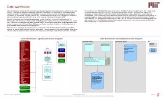
28. A three-tier DWH Architecture 1. Bottom Tier :- DWH server, is almost like a relational DB System. Back-end tools are used to fetch data from operational DB or external sources. These tools perform data cleaning, data extraction and transformation, load and refresh functions to update DWH. The data are extracted using API called as gateways(OLEBD, JDBE) which allows client programs to generate SQL code to be executed at server. • It also contains meta data repository to store information about DWH. 2. Middle Tier :- Ii is an OLAP server presents multidimensional data from DWH/Data Marts. It includes ROLAP/MOLAP/HOLAP servers. (i) ROLAP:- Use relational DBMS to store and manage warehouse data and include optimization of DBMS backend, implementation of aggregation navigation logic, and additional tools and services. Greater Scalability. Ex:- Informix, Informatica G.Karuna, GRIET

29. A three-tier DWH Architecture (ii) MOLAP:- It is a special purpose server that directly implements multidimensional model and operations with sparse array-based multidimensional storage engine. • It allows fast indexing to precomputed, summarized data. It uses sparse matrix compression techniques to store data Ex:- Essbase of Arbor (iii) HOLAP:- The hybrid OLAP servers combines both ROLAP & MOLAP. It uses the greater scalabitity of ROLAP and fast computation of MOLAP. Ex:- MS-SQL server 7.0 3. Top-Tier:- Is a client which contains query and reporting tools, analysis and/or data mining tools. G.Karuna, GRIET

30. Data Warehouse Back-End Tools and Utilities • Data extraction • get data from multiple, heterogeneous, and external sources • Data cleaning • detect errors in the data and rectify them when possible • Data transformation • convert data from legacy or host format to warehouse format • Load • sort, summarize, consolidate, compute views, check integrity, and build indicies and partitions • Refresh • propagate the updates from the data sources to the warehouse G.Karuna, GRIET

31. Metadata Repository • Meta data is the data defining warehouse objects. It stores: • Description of the structure of the data warehouse • schema, view, dimensions, hierarchies, derived data defn, data mart locations and contents • Operational meta-data • data lineage (history of migrated data and transformation path), currency of data (active, archived, or purged), monitoring information (warehouse usage statistics, error reports, audit trails) • The algorithms used for summarization • The mapping from operational environment to the data warehouse • Data related to system performance • warehouse schema, view and derived data definitions • Business data • business terms and definitions, ownership of data, charging policies G.Karuna, GRIET

32. Three tier DWH Architecture G.Karuna, GRIET

33. Three Data Warehouse Models • Enterprise warehouse • Collects all of the information about subjects spanning in entire organization. It provides corporate wide data, integrated from one/more operational/external sources. • It contains detailed, summarized data. The size from 100 gigabytes to terabytes. • Models implemented on mainframes, super computers etc. • To build model takes years and complex task. • Data Mart • It is a subset of corporate-wide data. Its scope is confined to specific, selected groups, such as marketing data mart. • These are implemented on low cost servers. • Takes weeks to build a model. • Independent vs. dependent (directly from DWH) data mart. G.Karuna, GRIET

34. Three Data Warehouse Models • Virtual warehouse • A set of views over operational databases. • For efficient query processing, only some of the possible summary views may be materialized. • Easy to build but requires excess capacity on operational databases. G.Karuna, GRIET

35. A Recommended Approach for DWH Development • Top-down – serves a systematic solution & minimizes integration problems. But it is expensive, lack of flexibility. • Bottom-up – provides flexibility, low cost and rapid development but integration is difficult. • In recommended Approach, (i) High level corporate model is defined (within short period) that provide corporate, consistent and integrated view of data among various subjects. This need to refined further development of enterprise DWH/ data mart. (ii) Data marts can be implemented parallel with DWH, based on same corporate model set. (iii) Distributed data marts can be constructed to integrate different DM’s. (iv) A multitier DWH is constructed where the enterprise is sole custodian of all WH data then it is distributed to various dependent data marts. G.Karuna, GRIET

36. Data Warehouse Development: A Recommended Approach Multi-Tier Data Warehouse Distributed Data Marts Enterprise Data Warehouse Data Mart Data Mart Model refinement Model refinement Define a high-level corporate data model G.Karuna, GRIET

37. Data Warehouse Implementation -Efficient Computation of data cubes (i) Compute Cube (ii) Materialization - Indexing OLAP Data (i) Bitmap Indexing (ii) Join Indexing • From Data warehousing to Data Mining - Data Warehouse Usage - From On-Line Analytical Processing (OLAP) to On Line Analytical Mining (OLAM) G.Karuna, GRIET

38. DWH Implementation (a) Efficient Computation of data cubes (i) Compute cube operator:- • Data cube can be viewed as a lattice of cuboids . • The bottom-most cuboid is the base cuboid • The top-most cuboid (apex) contains only one cell. • The total number of cuboids or groupby’s can be computed for data cube is 2n . • EX:- If dimensions given as item, city and year. 23 = 8 Queries: “ compute sum of sales group by city” “compute sum of sales group by city and item” G.Karuna, GRIET

39. () (city) (item) (year) (city, item) (city, year) (item, year) (city, item, year) DWH Implementation • compute cube operator computes aggregates overall subsets of dimensions specified in the opeartion. • The possible groupby’s are {(city, item, year), (city, item), (city, year), (item,year), (city), (item),(year),()} • Cube definition and computation in DMQL define cube sales[item, city, year]: sum(sales_in_dollars) compute cube sales G.Karuna, GRIET

40. DWH Implementation (ii) Materialization of data cube:- pre-computation of data cubes. There are 3 choices for materialization. • No Materialization:- Do not pre-compute any of the “nonbase” cuboids. This leads to computing expensive multidimensional aggregates on the fly, which can be extremely slow. • Full materialization: Pre-compute all of the cuboids. The resulting lattice of computed cuboids is referred to as the full cube. This choice typically requires huge amounts of memory space. • Partial materialization:Selectively compute a proper subset of the whole set of possible cuboids. Alternatively, we may compute a subset of the cube, which contains only some user-specified criterion. (i) identify the subset of cuboids to materialize (ii) exploit the materialized cuboids during query processing (iii) efficiently update the materialized cuboids during load and refresh G.Karuna, GRIET

41. DWH Implementation (b) Indexing OLAP Data:For efficient accessing most DWH systems support indexing. (i) Bit map Indexing:- This is an alternative representation of base table. It allows quick searching in data cube. In the bitmap index for a given attribute, there is a distinct bit vector, Bv, for each value v in the domain of the attribute. If the domain of a given attribute consists of n values, then n bits are needed for each entry in the bitmap index. G.Karuna, GRIET

42. DWH Implementation (ii) Join Indexing:- Join indexing registers the joinable rows of two relations from a relational database. Ex:- If two relations R(RID, A) and S(B, SID) join on the attributes A and B, then the join index record contains the pair (RID, SID), where RID and SID are record identifiers from the R and S relations, respectively. Hence, the join index records can identify joinable tuples. Join indexing is especially useful for maintaining the relationship between a foreign key and its matching primary keys, from the joinable relation. In DWH, join indexing is useful for cross table search because of star schema model of DWH. Join indexing maintains relationship between attribute values of dimension and the corresponding rows in fact table. G.Karuna, GRIET

43. DWH Implementation G.Karuna, GRIET

44. Efficient Methods for Data cube computation Data cube computation is an essential task in DWH. Pre-computation of all or part of a data cube can greatly reduce the response time and increase performance of OLAP. This is a challenging task. How can we compute data cubes in advance? Cube Materialization: (i) Base Cell:- A cell in base cuboid is base cell. (ii) Aggregate Cell:- A cell in non-base cuboid. Each aggregated dimension indicated as ‘*’. Ex:- If we take 3D-cube all 1-D, 2-D cells are aggregate cells and 3-D is Base cell. (iii) Ancestor & Descendent cells:- 1-D and 2-D cells are ancestors of 3-D cell. 3-D is descendent cell. G.Karuna, GRIET 44

45. Cube Materialization: Full Cube vs. Iceberg Cube Full cube:- Computation all the cells of all the cuboids in data cube. Iceberg cube:- Computing only the cuboid cells whose measure satisfies the iceberg condition. EX:- Only a small portion of cells may be “above the water’’ in a sparse cube compute cube sales iceberg as select month, city, customer group, count(*) from salesInfo cube by month, city, customer group having count(*) >= min support Closed Cube:-The cube consists of only closed cells. A cell that has no descendant cell than it is closed cell. G.Karuna, GRIET 45

46. Efficient Computation methods for data cube • Computing full/iceberg cubes: 3 methodologies (i) Bottom-Up: Multi-Way array aggregation (Zhao, Deshpande & Naughton, SIGMOD’97) (ii) Top-down: • BUC (Beyer & Ramarkrishnan, SIGMOD’99) (iii) Integrating Top-Down and Bottom-Up: • Star-cubing algorithm (Xin, Han, Li & Wah: VLDB’03) G.Karuna, GRIET 46

47. C c3 61 62 63 64 c2 45 46 47 48 c1 29 30 31 32 c 0 B 60 13 14 15 16 b3 44 28 56 9 b2 B 40 24 52 5 b1 36 20 1 2 3 4 b0 a0 a1 a2 a3 A Multi-way Array Aggregation for Cube Computation (MOLAP) • Partition arrays into chunks (a small subcube which fits in memory). • Compressed sparse array addressing: (chunk_id, offset) • Compute aggregates in “multiway” by visiting cube cells in the order which minimizes the # of times to visit each cell, and reduces memory access and storage cost. What is the best traversing order to do multi-way aggregation? G.Karuna, GRIET 47

48. Multi-Way Array Aggregation • Array-based “bottom-up” algorithm • Using multi-dimensional chunks • No direct tuple comparisons • Simultaneous aggregation on multiple dimensions. • The best order is the one that minimizes the memory requirement and reduced I/Os G.Karuna, GRIET 48

49. Data Mining: Concepts and Techniques

50. Multi-Way Array Aggregation for Cube Computation • Method: the planes should be sorted and computed according to their size in ascending order • Idea: keep the smallest plane in the main memory, fetch and compute only one chunk at a time for the largest plane • Limitation of the method: computing well only for a small number of dimensions • If there are a large number of dimensions, “top-down” computation and iceberg cube computation methods can be explored. G.Karuna, GRIET 50