Download
1 / 68
680 likes | 874 Vues
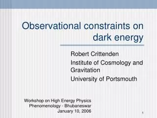
Observational constraints on dark energy. Robert Crittenden Institute of Cosmology and Gravitation University of Portsmouth. Workshop on High Energy Physics Phenomenology - Bhubaneswar January 10, 2006. SN: fainter than expected!.

E N D
Observational constraints on dark energy Robert Crittenden Institute of Cosmology and Gravitation University of Portsmouth Workshop on High Energy Physics Phenomenology - Bhubaneswar January 10, 2006
SN: fainter than expected! Is this because the universe is accelerating or due to a systematic? Dust, lensing, evolution Confirmed by many varied observations What drives it? “Dark energy” What might this dark energy be and how can we learn about it?
What drives the acceleration? • Cosmological constant • Introduced by Einstein to make a static universe. • Associated with a vacuum energy density, typically • It could be the Planck mass, or the super-symmetry or electro-weak breaking mass scale, but it is BIG. • Constant in space and time. • Equation of state:
What drives the acceleration? • Cosmological constant • Quintessence models • Motivated by models of inflation. • Scalar field rolling down shallow potential well. • Equation of state varies: • Smooth on small scales by repulsion, but clusters on scales larger than dark energy sound horizon scale. • Naturalness issues: • Why now?
Myriad of Quintessence models The equation of state is dynamic and depends on the precise choice of potential. Fundamental physics has not determined the functional form of the potential, much less the specific parameters. Like inflation, no preferred model! Albrecht & Weller
What drives the acceleration? • Cosmological constant • Quintessence models • Phantoms and ghosts • Any equation of state, • Can lead to ‘Big Rip’ divergences in finite times. • Violates weak and dominant energy conditions, and has negative energy states. • Classical and quantum instabilities. • Very difficult to find a working physical model.
What drives the acceleration? • Cosmological constant • Quintessence models • Phantoms and ghosts • Tangled defect networks Tangled string or domain wall networks give very specific predictions but are effectively ruled out observationally:
What drives the acceleration? • Cosmological constant • Quintessence models • Phantoms and ghosts • Tangled defect networks • Modification of gravity on large scales Many possible ideas: Branes, Brans-Dicke theories, MOND, backreaction of fluctuations?
What drives the acceleration? • Cosmological constant • Quintessence models • Phantoms and ghosts • Tangled defect networks • Modification of gravity on large scales What can the observational data tell us about the dark energy properties: its density, evolution and clustering?
Expansion rate H(z) • We have no evidence that dark energy interacts other than gravitationally. • It is believed to be smooth on small scales. • Thus, virtually our only handle on its nature is through its effect on the large scale expansion history of the universe, described by the Hubble parameter, H(z), and things which depend on it.
Observable effects of dark energy • It contributes to the present energy density and thus to the Hubble expansion rate. • It contributed to the past expansion rate, so affects the distance and time measurements to high redshifts. • It affects the growth rate of dark matter perturbations in two ways: • A faster expansion rate in the past would have made it harder for objects to collapse. • On large scales, the dark matter reacts to the perturbations in the dark energy.
CMB and large scale surveys What can these tell us about dark energy? Virtually all of the information is in their two point correlations, with themselves and with each other.
Power spectra These spectra describe the statistical properties of the maps and their features contain a great deal of information about the universe.
Weighing the universe There must be enough matter to explain the present expansion rate: Dark energy density we’re trying to determine
Weighing the universe There must be enough matter to explain the present expansion rate: • Dark matter density constraints (~25%): • CMB Doppler peak heights • Position of LSS turnover
Weighing the universe There must be enough matter to explain the present expansion rate: • Dark matter density constraints (~20-25%): • Baryon/dark matter ratio in x-ray clusters • Large scale velocities, mass/light ratio
Weighing the universe There must be enough matter to explain the present expansion rate: • Baryon density constraints (~4%): • Light element abundances • CMB Doppler peak ratios
Weighing the universe There must be enough matter to explain the present expansion rate: • Photon density constraint (0.004 %): • Observed CMB temperature
Weighing the universe There must be enough matter to explain the present expansion rate: • Neutrino density constraints (< 1%): • Small scale damping in LSS • Overall neutrino mass limits
Weighing the universe There must be enough matter to explain the present expansion rate: • Curvature of universe constraint (< 2%): • Angular size of CMB structures
Weighing the universe There must be enough matter to explain the present expansion rate: • Critical density constraint: • Measurement of Hubble constant • Biggest source of possible systematic errors
Weighing the universe There must be enough matter to explain the present expansion rate: Assuming value measured by Hubble Key Project, 70-75% of matter not observed. H0 = 72+-8 km/s/Mpc
Evolution of the expansion rate H(z) Evolution of dark energy determined by its equation of state: While the dark energy density is larger than the other components, it can be constrained by measuring the evolution of H(z). Changing H(z) effects distances and times to high redshifts.
Evolution of the expansion rate • Cosmic clocks Age of objects, now and at high redshifts: Weak constraints from globular cluster ages. Use luminous red galaxies as clocks if they evolve passively? Not all formed at the same time, so requires many high redshift galaxies to find the oldest.
Evolution of the expansion rate • Cosmic clocks • Co-moving volume If objects have constant co-moving density, then their number counts can constrain the expansion evolution Requires many high redshift galaxies and no density evolution. Constraints from strong gravitational lensing.
Evolution of the expansion rate • Cosmic clocks • Co-moving volume • Angular distance relation Angular size of distant objects can tell you how far away they are: Requires large yardstick of known size.
The baryon yardstick Before electrons and protons combined, they were tightly coupled to photons and so the density fluctuations oscillated acoustically. The largest scales which had time to compress before recombination were imprinted on the CMB and LSS power spectra Given and its angular size, we can find dA … if we know the curvature! Flat Closed
CMB as cosmic yardstick Both the curvature and the dark energy can change the scale of the Doppler peaks. We used the position of the Doppler peaks to determine the curvature, assuming a cosmological constant. However, if we assume a flat universe, we can turn this around to find a constraint on the equation of state. WMAP compilation Angular distance to last scattering surface
CMB angular distance Degeneracy needs to be broken by other data, like Hubble constant or SN data. Present data is consistent with w=-1, so we cannot change w too much, unless we compensate it by changing the curvature. Small amount of curvature keeps peak position unchanged Flat universe Recall DE slightly changes peak position Single integrated constraint on w and present density from the shape of CMB spectrum: w < -0.8. Lewis & Bridle 03 MCMC results
LSS as a cosmic yardstick Imprint of oscillations less clear in LSS spectrum unless high baryon density Detection much more difficult: • Survey geometry • Non-linear effects • Biasing Big pay-off: Potentially measure dA(z) at many redshifts! Eisenstein et al. 98
Baryon oscillations detected! SDSS data SDSS and 2dF detect baryon oscillations at 3-4 sigma level. SDSS detection in LRG sample z ~ 0.35 Thus far, fairly weak constraints on equation of state. Future: many competing surveys KAOS - Kilo-Aperture Optical Spectrograph, SKA ~106 galaxies at z = 0.5-1.3, z = 2.5-3.5
Evolution of the expansion rate • Cosmic clocks • Co-moving volume • Angular distance relation • Alcock-Paczynski tests Compare dimensions of objects parallel and perpendicular to the line of sight and ensure that they are the same on average.
Evolution of the expansion rate • Cosmic clocks • Co-moving volume • Angular distance relation • Alcock-Paczynski tests • Luminosity distance relation Use supernovae (or perhaps GRB’s) as standard candles and see how their brightness changes with their redshift.
Recent supernovae constraints ‘Gold’ data has best 150 SN and includes high redshift SN discovered with the Hubble telescope. Rules out ‘grey’ dust models. Residuals relative to an empty universe Riess et al. 2004
Recent supernovae constraints Limits on density and equation of state Riess et al. 2004
SNLS results New independent sample of 71 supernovae Astier et al. 2005
SNLS + baryon oscillations Combining data sets indicates close to cosmological constant with about 70% of the present density.
Growth rate of structure Accelerated expansion makes gravitational collapse more difficult Normalized to present, dark energy implies fluctuations were higher in the past This ignores d.e. clustering, reasonable on small scales.
Probes of(z) • Difficult to measure, even its present value (parameterized in 8) is subject to some debate (0.6 - 1.0?). • CMB amplitude provides early point of reference. • Gravitational lensing (Jain talk.) • Evolution of galaxy clustering, though tied up with bias! • Controls the number of collapsed objects, like clusters.
Cluster abundances If the statistics are Gaussian, the number of collapsed objects above a given threshold depends exponentially on the variance of the field. Press-Schecter Thus, the growth factor controls the number of clusters at a given redshift.
Cluster abundances We can observe these in x-rays or the CMB via the Sunyaev-Zeldovich effect. Normalizing to the present, a dark energy dominated universe will have many more objects at high redshifts. Unfortunately, we don’t measure the masses directly, which can complicate the cosmological interpretation. XCS clusters from K. Romer
Probes of(z) • Difficult to measure, even its present value (parameterized in 8) is subject to some debate (0.6 - 1.0?). • CMB amplitude provides early point of reference. • Gravitational lensing (Jain talk.) • Evolution of galaxy clustering, though tied up with bias! • Controls the number of collapsed objects, like clusters. • Induces very recent CMB anisotropies!
Recent CMB anisotropies While most CMB fluctuations are created at last scattering, some can be generated at low redshifts gravitationally via the ISW (linear) and Rees-Sciama (non-linear) effects: potential depth changes as cmb photons pass through gravitational potential traced by galaxy density The potential is constant for a matter dominated universe, but begins to evolve when the two dark energy effects modify the growth rate of the fluctuations.
Two uncorrelated CMB maps The CMB fluctuations we see are a combination of two uncorrelated pieces, one induced at low redshifts by a late time transition in the total equation of state. Early map, z~1000 Structure on many scales ISW map, z< 4 Mostly large scale features
large scale correlations ISW fluctuations tend to be on the very largest scales On small scales, positive and negative ISW effects will tend to cancel out. This leads to an enhancement of the large scale power spectrum The early and late power is fairly weakly correlated, so the power spectra add directly: WMAP best fit scale invariant spectrum
Observing the ISW effect in the cmb map, additional anisotropies should increase large scale power • Not observed in WMAP data • In fact, decrease is seen • why might this be? • cosmic variance • no ISW, still matter dominated • accidental cancellation • drop in large scale power • simple adiabatic scenario wrong
Correlations with the galaxy distribution The gravitational potential determines where the galaxies are and where the ISW fluctuations are created! Thus the galaxies and the CMB should be correlated. Most of the cross correlation arises on large or intermediate angular scales (>1degree). The CMB is well determined on these scales by WMAP, but we need large galaxy surveys. Can we observe this?
S. Boughn, RC 2004 cmb sky WMAP Galactic plane, centre removed most aggressive WMAP masking 68% of sky WMAP internal linear combination map (ilc) also Tegmark, de Oliveira-Costa & Hamilton map (no significant differences in resulting correlations) dominant source of noise to cross correlation is accidental correlations of cmb map with other maps
hard x-ray background HEAO-1 x-ray satellite 3 degree resolution 3-17 keV’s Flown in 1970’s • Removed nearby sources: • Cuts (leaving 33% of sky): • Galactic plane, centre removed • brightest point sources removed • Fits: • monopole, dipole • detector time drift • Galaxy • local supercluster Virtually all visible structures cleaned out
x-ray cmb correlation compare observed correlation to that with Monte Carlo cmb maps with WMAP power spectrum correlation detected at 2.5-3 sigma level, very close to that expected from ISW. dots: observed thin: Monte Carlos thick: ISW prediction (WMAP best fit model) errors highly correlated