Understanding Non-Gaussianity in Cosmic Microwave Background and Large Scale Structure
310 likes | 455 Vues
This presentation discusses the significance of non-Gaussianity (NG) in the context of the Cosmic Microwave Background (CMB) and high-redshift galaxy clusters. It explores the implications of observed Gaussianity in the CMB and considers how primordial fluctuations may challenge existing models of inflation. The talk highlights methods for testing Gaussianity, including null tests and model-testing approaches, while addressing the need for statistical tools that correlate with model parameters. The goal is to find compelling evidence for NG to shed light on the early universe.

Understanding Non-Gaussianity in Cosmic Microwave Background and Large Scale Structure
E N D
Presentation Transcript
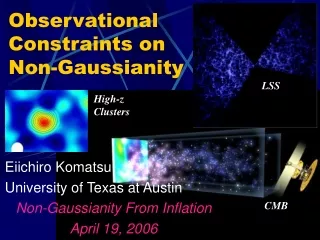
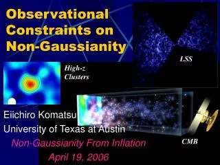
Observational Constraints on Non-Gaussianity LSS High-z Clusters Eiichiro Komatsu University of Texas at Austin Non-Gaussianity From Inflation April 19, 2006 CMB
Why Study NG? (Why Care?!) • Who said that CMB should be Gaussian? • Don’t let people take it for granted! • It is remarkable that the observed CMB is (very close to being) Gaussian. • The WMAP map, when smoothed to 1 degree, is entirely dominated by the CMB signal. • If it were still noise dominated, no one would be surprised that the map is Gaussian. • The WMAP data are telling us that primordial fluctuations are very close to being Gaussian. • How common is it to have something so close to being Gaussian in astronomy? E.g., Maxwellian velocity distribution, what else? • It may not be so easy to explain that CMB is Gaussian, unless we have a compelling early universe model that predicts Gaussian primordial fluctuations: Inflation. • “Gaussianity” should be taken as seriously as “Flatness”.
Gaussianity vs Flatness • People are generally happy that geometry of our Universe is flat. • 1-Wtotal=-0.003 (+0.013, -0.017) (68% CL) (WMAP03+HST) • Geometry of our Universe is consistent with being flat to ~3% accuracy at 95% CL. • What do we know about Gaussianity? • For F=FG+fNLFG2, -54<fNL<114 (95% CL) (WMAP03) • Primordial fluctuations are consistent with being Gaussian to ~0.001% accuracy at 95% CL. • In a way, inflation is supported more by Gaussianity of primordial fluctuations than by flatness. (Just kidding.)
Let’s Hunt Some NG! • The existing CMB data already suggest that primordial fluctuations are very close to being Gaussian; however, this does not imply, by any means, that they are perfectly Gaussian. • In fact, we would be in a big trouble if fNL turned out to be too close to zero. Second-order GR perturbations in the standard cosmological model must produce fNL~5 or so. (See Sabino Matarrese’s and Nicola Bartolo’s Talks, and Michelle Liguori’s Poster) • Some inflationary models produce much larger fNL. We may be able to distinguish candidate inflationary models by NG. (Not to mention that the simplest, single-field, slow-roll models produce tiny NG.) • The data keep getting better. • If we could find it, it would lead us to something huge.
Finding NG? • Two approaches to • I. Null (Blind) Tests / “Discovery” Mode • This approach has been most widely used in the literature. • One may apply one’s favorite statistical tools (higher-order correlations, topology, isotropy, etc) to the data, and show that the data are (in)consistent with Gaussianity at xx% CL. • PROS: This approach is model-independent. • CONS: We don’t know how to interpret the results. • “The data are consistent with Gaussianity” --- what physics do we learn from that? It is not clear what could be ruled out on the basis of this kind of test. • II. “Model-testing” Mode • Somewhat more recent approaches. • Try to constrain “NG parameter(s)” (e.g., fNL) • PROS: We know what we are testing, we can quantify our constraints, and we can compare different data sets. • CONS: Highly model-dependent. We may well be missing other important NG signatures.
Recent Tendency • I. Null (Blind) Tests / “Discovery” Mode • This approach is being applied mostly to the “large-scale anomaly” of the WMAP data. • North-south asymmetry • Quadrupole-octopole alignment • Some pixels are too cold (Marcos Cruz’s Poster) • “Axis of Evil” (Joao Magueijo’s Talk) • Large-scale modulation • II. “Model-testing” Mode • A few versions of fNL have been constrained using the bispectrum, Minkowski functionals and other statistical methods.
App. II: What Do We Need? • We need to know the predicted form of statistical toolsas a function of model parameters to fit the data. • For F=FG+fNLFG2, there are only three statistical tools for which the analytical predictions are known: • The angular bispectrum • Komatsu & Spergel (2001); Babich & Zaldarriaga (2004) • The angular trispectrum • Okamoto & Hu (2002); Kogo & Komatsu (2006) • Minkowski functionals • Hikage, Komatsu & Matsubara (2006)
Simplified Model: • Working assumption: fNL is independent of scales • Clearly an oversimplification! (Note, however, that this form is actually predicted from curvaton models and the non-linear Sachs-Wolfe effect in the large-scale limit.) • Why use this ansatz? Current observations are not yet sensitive to scale-dependence of fNL, but are only sensitive to the overall amplitude. • See Creminelli et al. (2005) for an alternative ansatz. • Sensitivity Goal: fNL~1 • Why fNL~1? NG “floor”: the ubiquitous signal from the second-order GR produces something like fNL~5, which would set the lower limit to which one may hope to detect the primordial non-Gaussianity. • It may be possible to achieve fNL~3 using the angular bispectrum from the Planck and CMBPol data. How do we go from there to fNL~1?
How Do They Look? Simulated temperature maps from fNL=0 fNL=100 fNL=1000 fNL=5000
Is One-point PDF Useful? Conclusion: 1-point PDF is not very useful. (As far as CMB is concerned.) A positive fNL yields negatively skewed temperature anisotropy.
Spergel et al. (2006) One-point PDF from WMAP • The one-point distribution of CMB temperature anisotropy looks pretty Gaussian. • Galaxy has been masked. • Left to right: Q (41GHz), V (61GHz), W (94GHz).
Angular Bispectrum, Blmn • A simple statistic that captures all of the information contained in the third-order moment of CMB anisotropy. • Theoretical predictions exist. • Statistical properties well understood.
Komatsu & Spergel (2001) How Does It Look? • Primordial • Inflation • Second-order PT • Secondary • Gravitational lensing • Sunyaev-Zel’dovich effect • Nuisance • Radio point sources • Our Galaxy
?Angular Bispectrum, Blmn? • Physical non-Gaussian signals should be generated in real space (via e.g., non-linear coupling), and thus should be more apparent in real space. • The Central Limit Theorem makes alm coefficients more Gaussian! • Non-Gaussianity localized in real space is obscured and spread over many l’s and m’s. • Challenges in the analysis • Sky cut complicates the analysis in harmonic space in many ways. • Computationally expensive (but not impossible). • 8 hours on 16 procs of an SGI Origin 300 for measuring all configurations up to l=512.
Komatsu, Spergel & Wandelt (2005) Optimal “Cubic” Statistics • Motivation • We know the shape of the angular bispectrum. • Find the “best statistic” in real space that is most sensitive to the kind of non-Gaussianity we are looking for. • Results • The statistics already combine all configurations of the bispectrum optimally. • Optimized just for fNL: Maximum adaptation of the approach II. • 1000 times faster for lmax=512 (30 sec vs 8 hours) • 4000 times faster for lmax=1024 (4 minutes vs 11 days) • One can also find an optimized statistics just for point sources.
Cubic Estimator = Skewness of Filtered Maps • B(x) is a Wiener reconstructed primordial potential field. • A(x) picks out relevant configurations of the bispectrum.
Wiener-reconstructed Primordial Curvature On the largest scale, Reconstruction can be made even better by including the polarization data. (See Ben Wandelt’s Talk)
Komatsu et al. (2006) It Works Very Well. • The statistics tested against simulations UNBIASED UNCORRELATED UNBIASED
Komatsu et al. (2003); Spergel et al. (2006) Bispectrum Constraints • Still far, far away from fNL~1, but it could put some interesting limits on parameters of curvaton models, ghost inflation, and DBI inflation models. (1yr) (3yr)
Angular Trispectrum, Tlmpq(L) • Why care?! Two reasons. • The trispectrum could be non-zero even when the bispectrum is exactly zero. • We may increase our sensitivity to primordial NG by including the trispectrum in the analysis.
Kogo & Komatsu (2006) Not For WMAP, But Perhaps For Planck… • Trispectrum (~ fNL2) is more sensitive than the bispectrum (~ fNL) when fNL is large. • At Planck resolution, the trispectrum would be detected more significantly than the bispectrum, if fNL > 50.
Minkowski Functionals • Morphology • Area • Contour length • Euler characteristics (or “Genus”) • The number of hot spots minus cold spots. • All quantities are evaluated as a function of the peak height relative to r.m.s.
Komatsu et al. (2003); Spergel et al. (2006) MFs from WMAP (1yr) (3yr) Area Contour Length Genus
Hikage, Komatsu & Matsubara (2006) Analytical Calculations • The analytical formulae should be very useful: we do not need to run NG simulations for doing MFs any more. • The formulae indicate that MFs are actually as sensitive to fNL as the bispectrum; however, MFs do not contain any more information than the bispectrum does.
Using Galaxies CIP • Not only CMB, but also the large-scale structure of the universe does contain information about primordial fluctuations on large scales. (See Peter Coles’s Talk.) • One example: Galaxy Bispectrum Cosmic Inflation Probe (CIP), a galaxy survey measuring 10 million galaxies at 3<z<6, would offer an opportunity to use this formula to constrain fNL~5 (note that the scale measured by CIP is smaller than that measured by CMB by a factor of ~10!)
Using High-z Objects • Massive objects forming at high-z are extremely rare: they form at high peaks of (nearly) Gaussian random field. • Even a slight distortion of a Gaussian tail can enhance (or reduce) the number of high-z object dramatically. The higher the mass is, or the higher the redshift is, the bigger the effect becomes.
Komatsu et al. (2003) Implications for high-z objects • The current WMAP limits still permit large changes in the number of objects at high z. • A golden object, like a few times 1014 solar masses at z=3, would be a smoking gun.
Summary • There have been a lot of development in this field, and there is still a lot more to do. It is timely to have a workshop that focuses on non-Gaussianity from Inflation! • We need more accurate predictions for the form of observables, such as the CMB bispectrum, trispectrum, Minkowski functionals, and others, from • Various models of inflation • Second-order PT, including second-order effects in Boltzmann equation • Not just CMB! • Galaxies and high-z objects might give us some surprises. • Toward the sensitivity goal, fNL~1. • What would be the best way to achieve this sensitivity? • Currently, the CMB bispectrum seems to be ahead of everything else. • The temperature plus polarization bispectrum would allow us to get down to fNL~3. How do we break this barrier? • Yet, the real surprise might come from the Approach I.