V. Homomorphic Signal Processing
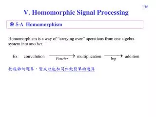
V. Homomorphic Signal Processing. 5-A Homomorphism. Homomorphism is a way of “carrying over” operations from one algebra system into another. Ex. convulution multiplication addition 把複雜的運算,變成 效能相同但 較簡單的運算. For the system D * [ . ] . 157.

V. Homomorphic Signal Processing
E N D
Presentation Transcript
V. Homomorphic Signal Processing 5-A Homomorphism Homomorphism is a way of “carrying over” operations from one algebra system into another. Ex. convulution multiplicationaddition 把複雜的運算,變成效能相同但較簡單的運算
For the system D*[.] 157 5-B Cepstrum convolution product addition addition + + * x[n] FT[.] Log[ ] FT-1[.] X(F) FT: discrete-time Fourier transform
由 y[n]= x[n]*h[n] 重建 x[n] x[n] y[n]= x[n]*h[n] * + + + + * D*[ ] Linear Filter D-1*[ ] For the system D-1*[.] 有趣的名詞 cepstrum quefrency lifter
5-C Complex Cepstrum and Real Cepstrum Complex Cepstrum ambiguity for phase Problems: (1) (2) Actually, the COMPLEX Cepstrum is REAL for real input
160 Real Cepstrum (but some problem of is not solved)
5-D Methods for Computing the Cepstrum Method 1: Compute the inverse discrete time Fourier transform: Problem: may be infinite
Method 2 (From Poles and Zeros of the Z Transform) 162 time delay where Poles & zeros inside unite circle Poles & zeros outside unite circle
163 Taylor series Z-1 (inverse Z transform) ?
164 Z-1 Taylor series expansion (Suppose that r = 0) Poles & zeros inside unit circle, right-sided sequence Poles & zeros outside unit circle, left-sided sequence Note: (1) 在 complex cepstrum domain Minimum phase 及 maximum phase 之貢獻以 n = 0 為分界切開 (2) For FIR case, ck = 0, dk = 0 (3) The complex cepstrum is unique and of infinite duration for both positive & negative n, even though x[n] is causal & of finite durations
Method 3 Z-1
Suppose that x[n] is causaland has minimum phase, i.e. x[n] = = 0, n < 0 For a minimum phase sequence x[n] 166
For anti-causal and maximum phase sequence, x[n] = = 0, n > 0 For maximum phase sequence, 167
5-E Properties P.1 ) The complex cepstrum decays at least as fast as P.2 ) If X(Z) has no poles and zeros outside the unit circle, i.e. x[n] is minimum phase, then because of no bk, dk P.3 ) If X(Z) has no poles and zeros inside the unit circle, i.e. x[n] is maximum phase, then because of no ak, ck
169 P.4 ) If x[n] is of finite duration, then has infinite duration
(1) Equalization for Echo 170 5-F Application of Homomorphic Deconvolution Let p[n] be p[n] =δ[n] +αδ[n-Np] x[n] =s[n] +αs[n-Np] =s[n] * p[n] Z-1
Filtering out the echo by the following “lifter”: (2) Representation of acoustic engineering x[n] = s[n] * h[n] Np 2Np 3Np Signal 171 n Synthesized music music building effect:eg. 羅馬大教堂的impulse response
(3) Speech analysis (4) Seismic Signals (5) Multiple-path problem analysis 172 Speech wave Pitch Global wave shape Vocal tract impulse They can be separated by filtering in the complex Cepstrum Domain
用cepstrum 將 pitch 的影響去除 173 From 王小川, “語音訊號處理”,全華出版,台北,民國94年。
175 5-G Problems of Cepstrum • (1) | log(X(Z))| • (2) Phase • (3) Delay Z-k • (4) Only suitable for the multiple-path-like problem
5-H Differential Cepstrum 或 inverse Z transform Note: If Advantages: no phase ambiguity able to deal with the delay problem
Properties of Differential Cepstrum (1) The differential Cepstrum is shift & scaling invariant 不只適用於 multi-path-like problem 也適用於 pattern recognition If y[n] = A X[n - r] (Proof):
(2) The complex cepstrum is closely related to its differential cepstrum and the signal original sequence x[n] Complex cepstrum 做得到的事情, differential cepstrum 也做得到!
(3) If x[n] is minimum phase (no poles & zeros outside the unit circle), then = 0 for n 0 (4) If x[n] is maximum phase (no poles & zeros inside the unit circle) , then = 0 for n 2 delay max phase min phase 0 1 2 179 (5) If x(n) is of finite duration, has infinite duration Complex cepstrum decay rate Differential Cepstrum decay rate 變慢了,
Take log in the frequency mask Bm[k] = 0 for k < fm1 and k > fm+1 for fm1ffm for fmffm+1 180 5-I Mel-Frequency Cepstrum (梅爾頻率倒頻譜) mask of Mel-frequency cepstrum gain frequency fm-1 fm fm+1
x[n] X[k] Q: What are the difference between the Mel-cepstrum and the original cepstrum? Mel-frequency cepstrum 更接近人耳對語音的區別性 用 cx[1], cx[2], cx[3], ……., cx[13] 即足以描述語音特徵 181 Process of the Mel-Cepstrum FT summation of the effect inside the mth mask
R. B. Randall and J. Hee, “Cepstrum analysis,” Wireless World., vol. 88, pp. 77-80. Feb. 1982 王小川, “語音訊號處理”,全華出版,台北,民國94年。 A. V. Oppenheim and R. W. Schafer, Discrete-Time Signal Processing, London: Prentice-Hall, 3rd ed., 2010. S. C. Pei and S. T. Lu, “Design of minimum phase and FIR digital filters by differential cepstrum,” IEEE Trans. Circuits Syst.I, vol. 33, no. 5, pp. 570-576, May 1986. S. Imai, “Cepstrum analysis synthesis on the Mel-frequency scale,” ICASSP, vol. 8, pp. 93-96, Apr. 1983. 182 5-J References
183 附錄六:聲音檔和影像檔的處理 (by Matlab) A. 讀取聲音檔 • 電腦中,沒有經過壓縮的聲音檔都是 *.wav 的型態 • 讀取: wavread • 例: [x, fs] = wavread('C:\WINDOWS\Media\ringin.wav'); 可以將 ringin.wav 以數字向量 x來呈現。 fs: sampling frequency 這個例子當中 size(x) = 9981 1 fs = 11025 • 思考: 所以,取樣間隔多大? • 這個聲音檔有多少秒?
184 畫出聲音的波型 time = [0:length(x)-1]/fs; % x 是前頁用 wavread 所讀出的向量 plot(time, x) 注意: *.wav 檔中所讀取的資料,值都在 1 和 +1 之間
185 • 一個聲音檔如果太大,我們也可以只讀取它部分的點 • [x, fs]=wavread('C:\WINDOWS\Media\ringin.wav', [4001 5000]); • % 讀取第4001至5000點 [x, fs, nbits] = wavread('C:\WINDOWS\Media\ringin.wav'); nbits: x(n) 的bit 數 • 第一個bit : 正負號,第二個bit : 21,第三個bit : 22, ….., • 第 n 個bit : 2nbits +1, 所以 x乘上2nbits 1是一個整數 • 以鈴聲的例子, nbits = 8,所以 x 乘上 128是個整數
186 • 有些聲音檔是 雙聲道 (Stereo)的型態 (俗稱立體聲) 例: [x, fs]=wavread('C:\WINDOWS\Media\notify.wav'); • size(x) = 29823 2 fs = 22050
187 B. 繪出頻譜 (請參考附錄四) X = fft(x);plot(abs(X)) fft 橫軸 轉換的方法 (1) Using normalized frequency F: F = m / N. (2) Using frequency f, f = F fs= m (fs / N).
189 C. 聲音的播放 (1) wavplay(x): 將 x以 11025Hz 的頻率播放 (時間間隔 = 1/11025 = 9.07 105秒) (2) sound(x): 將 x以 8192Hz 的頻率播放 (3) wavplay(x, fs) 或 sound(x, fs): 將 x以 fs Hz 的頻率播放 Note: (1)~(3) 中 x必需是1 個column (或2個 columns),且 x的值應該 介於 1 和 +1 之間 (4) soundsc(x, fs): 自動把 x的值調到 1 和 +1 之間 再播放
190 D. 用 Matlab 製作 *.wav 檔: wavwrite wavwrite(x, fs, waveFile) 將數據 x變成一個 *.wav 檔,取樣速率為 fs Hz x必需是1 個column (或2個 columns) x值應該 介於 1 和 +1 之間 若沒有設定fs,則預設的fs 為 8000Hz
191 E. 用 Matlab 錄音的方法 錄音之前,要先將電腦接上麥克風,且確定電腦有音效卡 (部分的 notebooks 不需裝麥克風即可錄音) 範例程式: Sec = 3; Fs = 8000; recorder = audiorecorder(Fs, 16, 1); recordblocking(recorder, Sec); audioarray = getaudiodata(recorder); 執行以上的程式,即可錄音。 錄音的時間為三秒,sampling frequency 為 8000 Hz 錄音結果為 audioarray,是一個 column vector (如果是雙聲道,則是兩個 column vectors)
192 範例程式 (續): wavplay(audioarray, Fs); % 播放錄音的結果 t = [0:length(audioarray)-1]./Fs; plot (t, audioarray‘); % 將錄音的結果用圖畫出來 xlabel('sec','FontSize',16); wavwrite(audioarray, Fs, ‘test.wav’) % 將錄音的結果存成 *.wav 檔
193 指令說明: recorder = audiorecorder(Fs, nb, nch); (提供錄音相關的參數) Fs: sampling frequency, nb: using nb bits to record each data nch: number of channels (1 or 2) recordblocking(recorder, Sec); (錄音的指令) recorder: the parameters obtained by the command “audiorecorder” Sec: the time length for recording audioarray = getaudiodata(recorder); (將錄音的結果,變成 audioarray 這個 column vector,如果是雙聲道,則 audioarray 是兩個 column vectors) 以上這三個指令,要並用,才可以錄音
194 F:影像檔的處理 Image 檔讀取: imread Image 檔顯示: imshow, image, imagesc Image 檔製作: imwrite 基本概念:灰階影像在 Matlab 當中是一個矩陣 彩色影像在 Matlab 當中是三個矩陣,分別代表 Red, Green, Blue *.bmp: 沒有經過任何壓縮處理的圖檔 *.jpg: 有經過 JPEG 壓縮的圖檔 Video 檔讀取: aviread
範例一: (黑白影像) 195 im=imread('C:\Program Files\MATLAB\pic\Pepper.bmp'); (注意,如果 Pepper.bmp 是個灰階圖,im 將是一個矩陣) size(im) ans = 256 256 (用 size 這個指令來看 im 這個矩陣的大小) image(im); colormap(gray(256)) 範例二:(彩色影像) im2=imread('C:\Program Files\MATLAB\pic\Pepper512c.bmp'); size(im2) ans = 512 512 3 (注意,由於這個圖檔是個彩色的,所以 im2 將由三個矩陣複合而成) imshow(im);