Probabilistic Robotics: Motion Model/EKF Localization
Advanced Mobile Robotics. Probabilistic Robotics: Motion Model/EKF Localization. Dr. J izhong Xiao Department of Electrical Engineering CUNY City College jxiao@ccny.cuny.edu. Robot Motion. Robot motion is inherently uncertain. How can we model this uncertainty?. Bayes Filter Revisit.

Probabilistic Robotics: Motion Model/EKF Localization
E N D
Presentation Transcript
Advanced Mobile Robotics Probabilistic Robotics: Motion Model/EKF Localization Dr. Jizhong Xiao Department of Electrical Engineering CUNY City College jxiao@ccny.cuny.edu
Robot Motion • Robot motion is inherently uncertain. • How can we model this uncertainty?
Bayes Filter Revisit • Prediction (Action) • Correction (Measurement)
Probabilistic Motion Models • To implement the Bayes Filter, we need the transition model p(xt| xt-1, u). • The term p(xt| xt-1, u) specifies a posterior probability, that action u carries the robot from xt-1 to xt. • In this section we will specify, how p(xt| xt-1, u) can be modeled based on the motion equations.
Coordinate Systems • In general the configuration of a robot can be described by six parameters. • Three-dimensional cartesian coordinates plus three Euler angles pitch, roll, and tilt. • Throughout this section, we consider robots operating on a planar surface. • The state space of such systems is three-dimensional (x, y, ).
Typical Motion Models • In practice, one often finds two types of motion models: • Odometry-based • Velocity-based (dead reckoning) • Odometry-based models are used when systems are equipped with wheel encoders. • Velocity-based models have to be applied when no wheel encoders are given. • They calculate the new pose based on the velocities and the time elapsed.
Example Wheel Encoders These modules require +5V and GND to power them, and provide a 0 to 5V output. They provide +5V output when they "see" white, and a 0V output when they "see" black. These disks are manufactured out of high quality laminated color plastic to offer a very crisp black to white transition. This enables a wheel encoder sensor to easily see the transitions. Source: http://www.active-robots.com/
Dead Reckoning • Derived from “deduced reckoning.” • Mathematical procedure for determining the present location of a vehicle. • Achieved by calculating the current pose of the vehicle based on its velocities and the time elapsed. • Odometry tends to be more accurate than velocity model, • But, Odometry is only available after executing a motion command, cannot be used for motion planning
different wheeldiameters carpet bump ideal case Reasons for Motion Errors and many more …
Odometry Model • Robot moves from to . • Odometry information . Relative motion information, “rotation” “translation” “rotation”
The atan2 Function • Extends the inverse tangent and correctly copes with the signs of x and y.
Noise Model for Odometry • The measured motion is given by the true motion corrupted with independent noise.
Typical Distributions for Probabilistic Motion Models Normal distribution Triangular distribution
Calculating the Probability (zero-centered) • For a normal distribution • For a triangular distribution • Algorithm prob_normal_distribution(a, b): • return • Algorithm prob_triangular_distribution(a,b): • return
odometry values (u) values of interest (xt-1, xt) Calculating the Posterior Given xt, xt-1, and u An initial pose Xt-1 A hypothesized final pose Xt A pair of poses u obtained from odometry • Algorithm motion_model_odometry (xt, xt-1, u) • return p1 · p2 · p3 Implements an error distribution over a with zero mean and standard deviation b
Application • Repeated application of the sensor model for short movements. • Typical banana-shaped distributions obtained for 2d-projection of 3d posterior. p(xt| u, xt-1) x’ x’ u u Posterior distributions of the robot’s pose upon executing the motion command illustrated by the solid line. The darker a location, the more likely it is.
Velocity-Based Model Rotation radius control
Equation for the Velocity Model Instantaneous center of curvature (ICC) at (xc , yc) Initial pose Keeping constant speed, after ∆t time interval, ideal robot will be at Corrected, -90
Velocity-based Motion Model With and are the state vectors at time t-1 and t respectively The true motion is described by a translation velocity and a rotational velocity Motion Control with additive Gaussian noise Circular motion assumption leads to degeneracy , 2 noise variables v and w 3D pose Assume robot rotates when arrives at its final pose
Velocity-based Motion Model Motion Model: 1 to 4 are robot-specific error parameters determining the velocity control noise 5 and 6 are robot-specific error parameters determining the standard deviation of the additional rotational noise
Probabilistic Motion Model How to compute ? Move with a fixed velocity during ∆t resulting in a circular trajectory from to Center of circle: with Radius of the circle: Change of heading direction: (angle of the final rotation)
Posterior Probability for Velocity Model Center of circle Radius of the circle Change of heading direction Motion error: verr ,werr and
Approximation: Map-Consistent Motion Model Obstacle grown by robot radius Map free estimate of motion model “consistency” of pose in the map “=0” when placed in an occupied cell
Summary • We discussed motion models for odometry-based and velocity-based systems • We discussed ways to calculate the posterior probability p(x| x’, u). • Typically the calculations are done in fixed time intervals t. • In practice, the parameters of the models have to be learned. • We also discussed an extended motion model that takes the map into account.
Localization, Where am I? • Given • Map of the environment. • Sequence of measurements/motions. • Wanted • Estimate of the robot’s position. • Problem classes • Position tracking (initial robot pose is known) • Global localization (initial robot pose is unknown) • Kidnapped robot problem (recovery)
Markov Localization Markov Localization: The straightforward application of Bayes filters to the localization problem
Bayes Filter Revisit • Prediction (Action) • Correction (Measurement)
EKF Linearization First Order Taylor Expansion • Prediction: • Correction:
EKF Algorithm • Extended_Kalman_filter( mt-1,St-1, ut, zt): • Prediction: • Correction: • Returnmt,St
EKF_localization ( mt-1,St-1, ut, zt,m):Prediction: Jacobian of g w.r.t location Jacobian of g w.r.t control Motion noise covariance Matrix from the control Predicted mean Predicted covariance
Velocity-based Motion Model With and are the state vectors at time t-1 and t respectively The true motion is described by a translation velocity and a rotational velocity Motion Control with additive Gaussian noise
Velocity-based Motion Model Motion Model:
Velocity-based Motion Model Derivative of g along x’ dimension, w.r.t. x at Jacobian of g w.r.t location
Velocity-based Motion Model Mapping between the motion noise in control space to the motion noise in state space Jacobian of g w.r.t control Derivative of g w.r.t. the motion parameters, evaluated at and
EKF_localization ( mt-1,St-1, ut, zt,m):Correction: Predicted measurement mean Jacobian of h w.r.t location Pred. measurement covariance Kalman gain Updated mean Updated covariance
Feature-Based Measurement Model • Jacobian of h w.r.t location Is the landmark that corresponds to the measurement of
EKF Localizationwith unknown correspondences Maximum likelihood estimator
UKF Localization • Given • Map of the environment. • Sequence of measurements/motions. • Wanted • Estimate of the robot’s position. • UKF localization
Unscented Transform Sigma points Weights Pass sigma points through nonlinear function For n-dimensional Gaussian λ is scaling parameter that determine how far the sigma points are spread from the mean If the distribution is an exact Gaussian, β=2 is the optimal choice. Recover mean and covariance
Motion noise UKF_localization ( mt-1,St-1, ut, zt,m): Prediction: Measurement noise Augmented state mean Augmented covariance Sigma points Prediction of sigma points Predicted mean Predicted covariance
Measurement sigma points UKF_localization ( mt-1,St-1, ut, zt,m): Correction: Predicted measurement mean Pred. measurement covariance Cross-covariance Kalman gain Updated mean Updated covariance