Download
1 / 30
300 likes | 432 Vues
Scheduling Data Broadcast in Asymmetric Communication Environment. Nitin H. Vaidya, Sohail Hameed CS Dept of Texas A&M University. Presented by Jianping Wang. Summary. Problem to be solved Module and objective Single broadcast channel Overall mean access time On-line scheduling algorithm

E N D
Scheduling Data Broadcast in Asymmetric Communication Environment Nitin H. Vaidya, Sohail Hameed CS Dept of Texas A&M University Presented by Jianping Wang
Summary • Problem to be solved • Module and objective • Single broadcast channel • Overall mean access time • On-line scheduling algorithm • On-line scheduling algorithm with bucketing • Effect of transmission errors • Multiple broadcast channels • Performance evaluation
Asymmetric Communication Environment Server has much more bandwidth than clients. It is not possible (or desirable) for clients to send explicit requests to the server. In this case, broadcasting the information is an effective way of making the information available simultaneously to a large number of users.
The Module and Objective Server have M information items to broadcast. Item i has length li which requires li time units to broadcast. The probability that item i is requested in any request is pi (Demand Probability ). The arrival of requests is governed by a Possion process. Objective: To find a broadcast schedule which consists of a cycle of size N time units. And the found schedule has the minimum Overall Mean Access Time.
The Definition of Terms • Frequency of an item i (fi): is the number of instances of item i in the broadcast cycle. • Access time: the time a client has to wait for some information it needs. • Instance of an item: an appearance of an item in the broadcast. • Spacing: the spacing between two instances of an item is the time it takes to broadcast from the beginning of the first instance to the beginning of the second instance. • Item mean access time (ti): The average access time among all clients which request item i. By assumption, if all instances of item i are equally spaced with spacing si, then ti = si/2. • Overall mean access time (t): t = =
An Example of Spacing Spacing between two instances of Item 1 10 8 4 10 7 Item 1 Item 2 Item 3 Item 1 Item 4 an instance of Item 1 an instance of Item 1
Mean Access Time • Let sij denotes the spacing between j-th instance of item i and the next instance of item i (1 ≤ j ≤ fi). We have: When sij = si(1 ≤ j ≤ fi), ti = si/2. When sij = si(1 ≤ j ≤fi), .
Two Important Results Lemma 1: The broadcast schedule with minimum overall mean access time results when the instances of each item are equally spaced. Theorem 1(Square-root Rule): Given demand probability pi of each item i, the minimum overall mean access time t, is achieved when frequency fi of each item i is proportional to and inversely proportional to , assuming that instances of each item are equally spaced. That is, Therefore, More specific,
The Optimal Overall Mean Access Time toptimal represents a lower bound on achievable overall mean access time. It is derived by assuming that instances of each item are equally spaced. (but does not require the spacings of two different items are identical) It is not achievable in general. But the results in the evaluation part of this paper show that the algorithms proposed in this paper can achieve performance almost identical to the above lower bound.
On-line Scheduling Algorithm From Therem 1, Define: Here Q is the current time, R(j) is the time at which an instance of item j was most recently transmitted. Algorithm A: On-line algorithm Step 1: Find Gmax = max{G(j), 1 ≤ j ≤ M}. Step 2: Choose i such that G(i) = Gmax. If find multiple i, select one of them randomly. Step 3: Broadcast item i at time Q. Step 4. R(i) = Q.
Theoretical optimal spacing of item 1 Item 1 Item 1 an instances of Item 1 R(1) Q T1 is increasing function of Q when
Encounter Example On-line scheduling algorithm is not always optimal. Example: 1 2 1 2 1 In this case, On-line scheduling algorithm produces cyclic schedule (1,2,1,2,…). The overall mean access time is 1. On the other hand, cyclic schedule (1,2,2,1,2,2,…) has overall mean access time 2.9/3 + 2ε/3 < 1.
On-line Algorithm with Bucketing (1/3) M items are divided into k buckets. Let bucket j contains mj items. Define: In this case, for optimality, the following condition holds: In other words,
On-line Algorithm with Bucketing (2/3) Define: Here Ijis the item at the front of bucket Bj. Algorithm B: On-line algorithm with Bucketing Step 1: Find Gmax = max{G(j), 1 ≤ j ≤ k}. Step 2: Choose i such that G(i) = Gmax. If find multiple i, select one of them randomly. Step 3: Broadcast item Iiat time Q. Step 4: Move item Ii from the front of the bucket Bi to the end. Step 5: R(Ii) = Q. Time complexity is reduced to O(k). The Optimal Overall Mean Access Time is:
On-line Algorithm with Bucketing (3/3) To carry out bucketing algorithm, M items can be divided into k buckets in the following way: Amin Amax Bucket Bk Bucket B1 Bucket B2
Effect of Transmission Errors (1/2) Suppose that uncorrectable errors occur in an item of length l with probability E(l). Assume the instances of item i are equally spaced with spacing si, the overall mean access time is: Theorem 2: The overall mean access time is minimized when and
Effect of Transmission Errors (2/2) In this case, the minimum overall mean access time is: Theorem 2 implies that in a optimal schedule, In the case of errors, algorithm A is also available when re-defining:
Multiple Broadcast Channels (1/3) Assume all items are transmitted on each channel. Partition items into different channels may cause starvation problem. Two Eaxmples: Channel 1 1 2 3 4 1 2 3 4 1 Channel 2 3 4 1 2 3 4 1 2 3 Channel 1 1 2 1 2 1 2 1 2 1 Channel 2 3 4 3 4 3 4 3 4 3
Multiple Broadcast Channels (2/3) H = {1,2,…c} - the set of all broadcast. A client may listen to any non-empty subset S of set H with probability . The overall mean access time for multi-channel broadcast is: A lower bound on tmultichan is given by:
Multiple Broadcast Channels (3/3) Let Rh(j) denote the most recent time when item j was broadcast on channel h (1≤h≤c, 1≤j≤M). For a subset S, define: Define: On-line algorithm for channel h, 1≤h≤c: Step 1: Step 2: Find Gmax = max{Gh(j), 1≤j≤k}. Step 3: Choose i such that Gh(i) = Gmax. If find multiple i, select one of them randomly. Step 4: Broadcast item i on channel h at time Q Step 5: Rh(i) = Q.
Performance Evaluation The number of items M = 1000, experiment time = 2,000,000 time units. Demand probabilities follow the Zipf distribution: θis access skew coefficient. Whenθ = 0, Zipf distribution reduces to uniform distribution. Item length distribution: • Uniform length distribution (L0=L1=1). • Increasing length distribution (L0=1, L1=10). • Increasing length distribution (L0=10, L1=1). • Also consider random length distribution in [1, 10].
Zipf distribution for various values of θ Length distribution larger θ brings larger differences in the access probability of all items.
Performance Evaluation in the Absence of Uncorrectable Errors The curve of algorithm A overlaps optimal curve. The simulation results are within 0.5% of analytical results. Bucketing algorithm can significantly reduce time complexity with only small performance degradation.
Performance Evaluation in the Presence of Uncorrectable Errors Assume uncorrectable errors follow an Poison process: When lengths follow uniform distribution, In this case, Theorem 2 reduces to Theorem 1.
The simulation results are within 2.5% of analytical results.
The simulation results are within 1.1% of analytical results.
Performance With Multiple Broadcast Channels The simulation results are within 1.0% of analytical results.
Comments: • All results are obtained based on strict statistical assumptions. • No analysis on the “close level” between on-line algorithms and theoretical results. • The analysis is based on broadcast cycle assumption but it is hard to find and use it in practices.