Download
1 / 48
480 likes | 583 Vues
This document outlines the current readiness of the LHC experiments' software, covering the startup progress, status as of the last CHEP conference, common software applications, deployment strategies, and remaining tasks. It highlights key areas such as the LHC startup plan, pilot run details, ALICE startup physics, and the overall startup plan and software requirements. The text provides insights into the evolving software landscape related to high-energy physics experiments like ALICE, CMS, ATLAS, and LHCb.

E N D
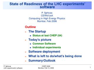
State of Readiness of the LHC experiments’ software Outline • The Startup • Status at last CHEP (04) • Today’s picture • Common Software • Individual experiments • Software deployment • What is left to do/what’s being done • Summary/Outlook P. Sphicas CERN/UoA Computing in High Energy Physics Mumbai, Feb 2006 CHEP 2006
LHC startup plan Stage 1 Initial commissioning 43x43 to 156x156, N=3x10¹⁰ Zero to partial squeeze L=3x1028 - 2x1031 Stage 2 75 ns operation 936x936, N=3-4x10¹⁰ partial squeeze L=1032 - 4x1032 Stage 3 25 ns operation 2808x2808, N=3-5x10¹⁰ partial to near full squeeze L=7x1032 - 2x1033 CHEP 2006
Higgs (?) Susy - Susy Z’ muons Top re-discovery LHC startup: CMS/ATLAS • Integrated luminosity with the current LHC plans Lumi (cm-2s-1) 1.9 fb-1 1033 1 fb-1 (optimistic?) 1032 1031 LHC = 30% (optimistic!) CHEP 2006
Pilot Run • Pilot Run : Luminosity • 30 days; maybe less (?); 43*43 bunches, then 156*156 bunches Int. Lumi (pb-1) Pile-up Lumi (cm-2s-1) 1031 10 1030 1 0.1 1029 1028 LHC = 20% (optimistic!) CHEP 2006
Startup physics (ALICE) Can publish two papers 1-2 weeks after LHC startup • Multiplicity paper: • Introduction • Detector system • - Pixel (& TPC) • Analysis method • Presentation of data • - dN/dη and mult. distribution (s dependence) • Theoretical interpretation • - ln2(s) scaling?, saturation, multi-parton inter… • Summary • pT paper outline: • Introduction • Detector system • - TPC, ITS • Analysis method • Presentation of data • - pT spectra and pT-multiplicity correlation • Theoretical interpretation • - soft vs hard, mini-jet production… • Summary CHEP 2006
Startup plan • Physics rush: • ALICE: minimum-bias proton-proton interactions • Standard candle for the heavy-ion runs • LHCb: BS mixing, sin2b repeat • If the Tevatron has not done it already • ATLAS-CMS: measure jet and IVB production; In 15 pb-1 will have 30K W’s and 4K Zs into leptons. • Measure cross sections and W and Z charge asymmetry (pdfs; IVB+jet production; top!) • Luminosity? CHEP 2006
Turn-on is fast Pile-up increasing rapidly Timing (43x43 to 75ns to 25 ns) evolution LOTS of physics For all detectors: Commission detector and readout Commission trigger systems Calibrate/align detector(s) Commission computing and software systems Rediscover the Standard Model Simulation Reconstruction Trigger Monitoring Calibration/Alignment calculation application User-level data objects selection Analysis Documentation Startup plan and Software Need it all CHEP 2006
Status at last CHEP F. Gianotti @ CHEP04 2007 My very rough estimate … average over 4 experiments • Realistic detectors (HV problems, dead channels, • mis-alignments, …) not yet implemented • Calibration strategy : • -- where (Event Filter, Tier0) ? • -- which streams, which data size ? • -- how often, how many reprocessings of part of raw data ? C PU ? • not fully developed in most cases • (implications for EDM and Computing Model ?) • Software for experiment monitoring and for • commissioning with cosmic and beam-halo muons • (the first real data to be collected …) not developed yet • (reconstruction must cope with atypical events …) Path accomplished (%) CHEP 2006
Today’s picture Common Software
LCG Application Area • Deliver the common physics applications software for the LHC experiments • Organized to ensure focus on real experiment needs • Experiment-driven requirements and monitoring • Architects in management and execution • Open information flow and decision making • Participation of experiment developers • Frequent releases enabling iterative feedback • Success is defined by adoption and validation of the products by the experiments • Integration, evaluation, successful deployment CHEP 2006
AA Projects • SPI – Software process infrastructure • Software and development services: external libraries, savannah, software distribution, support for build, test, QA, etc. • ROOT – Core Libraries and Services • Foundation class libraries, math libraries, framework services, dictionaries, scripting, GUI, graphics, SEAL libraries, etc. • POOL – Persistency Framework • Storage manager, file catalogs, event collections, relational access layer, conditions database, etc. • SIMU - Simulation project • Simulation framework, physics validation studies, MC event generators, Garfield, participation in Geant4 and Fluka. CHEP 2006
AA Highlights • SPI is concentrating on the following areas: • Savannah service (bug tracking, task management, etc.) • >160 hosted projects, >1350 registered users (doubled in one year) • Software services (installation and distribution of software) • >90 external packages installed in the external service • Software development service • Tools for development, testing, profiling, QA • Web and Documentation • ROOT activity at CERN fully integrated in the LCG organization (planning, milestones, reviews, resources, etc.) • The main change during last year has been the merge of the SEAL and ROOT projects • Single development team • Adiabatic migration of the software products into a single set of core software libraries • 50% of the SEAL functionality has been migrated into ROOT (mathlib, reflection, python scripting, etc.) • ROOT is now at the “root” of the software for all the LHC experiments CHEP 2006
AA Highlights (2) • POOL (object storage and references) has been consolidated • Adapted to new Reflex dictionaries, 64bit support, new file catalog interfaces, etc. • CORAL is a major re-design of the generic relational database access interface • Focusing on the deployment of databases in the grid environment • COOL conditions database is being validated • Many significant performance and functionality improvements • Currently being validated by ATLAS and LHCb • Consolidation of the Simulation activities • Major release of Fluka-2005.6 released in July 2005 • Garfield (simulation of gaseous detectors) added in the project scope • New developments and improvements of Geant4 toolkit • New results in the physics validation of Geant4 and Fluka CHEP 2006
Today’s picture Individual experiments
Converter Converter Application Manager Converter Transient Event Store Data Files Message Service Persistency Service Event Data Service JobOptions Service Algorithm Algorithm Algorithm Data Files Transient Detector Store Particle Prop. Service Persistency Service Detec. Data Service Other Services Data Files Transient Histogram Store Persistency Service Histogram Service Frameworks: essentially done • ALICE: AliROOT; ATLAS+LHCb: Athena/Gaudi • CMS: moved to a new framework; in progress CHEP 2006
ALICE : ~3 million volumes Simulation (I) • Geant4: success story; Deployed by all experiments. • Functionality essentially complete. Detailed physics studies performed by all experiments. • Very reliable in production (better than 1:104) • Good collaboration between experiments and Geant4 team • Lots of feedback on physics (e.g. from testbeams) • LoH (Level of Happiness): very high LHCb : ~ 18 million volumes CHEP 2006
CMS HCAL: Brass/Scintillator ATLAS Tilecal: Fe/Scintillator Simulation (II) • Tuning to data: ongoing. Very good progress made Geant4 / data for e/p CHEP 2006
Fast simulation (I) • Different levels of “fast” simu at the four expts: • CMS extreme: swimming particles through detector; include material effects, radiation, etc. Imitate full simulation – but much faster (1Hz). • ATLAS: particle-level smearing. VERY fast (kHz) • LHCb: generator output directly accessible by the physics application programs • But: ongoing work in bridging the gap • For example, in shower-parametrization in the G4 full simulation (ATLAS) • Common goal of all: output data at AOD level CHEP 2006
Fast simulation (II) Detailed geometry Complicated geometry, Propagation in short steps, full & slow simulation - t t Simplified (FAMOS) geometry Nested cylinders, Fast propagation, Fast material effect simulation. pT (2nd jet) CHEP 2006
Reconstruction, Trigger, Monitoring • General feature: all based on corresponding framework (AliRoot, Athena, Gaudi, CMSSW) • Multi-threading is necessary for online environment • Most Algorithms & Tools are common with offline • Two big versions: • Full reconstruction • “seeded”, or “partial”, or “reconstruction inside a region of interest” • This one used in HLT • Online monitoring and event displays • “Spying” on Trigger/DAQ data online • But also later in express analysis • Online calibrations CHEP 2006
Online selection CHEP 2006
High-Level Trigger • A huge challenge; large (small) rejection (accept) factor • In practice: startup will use smaller rates. • CMS example: 12.5 kHz (pilot run) and 50 kHz (1033 cm-2s-1) • Real startup conditions (beam, backgrounds, expt) unknown • Startup trigger tables: in progress. ATLAS/CMS have prototypes. Real values: when beam comes… Lvl-1 (HW) HLT (SW) CHEP 2006
Regional reco example: CMS HLT electrons (I) “Lvl-2” electron: recluster Inside extended Lvl-1 trigger area Brem recovery: “supercluster” Seed; road in f around seed; collect all clusters in road Add pixel information Very fast; pre-brem CHEP 2006
RZ VeloSpace Velo Long track Velo-TT Regional reco example: CMS HLT electrons (II) • “Level-3” selection • Full tracking, loose track-finding (to maintain high efficiency): • Cut on E/p everywhere, plus • Matching in h (barrel) • H/E (endcap) • Another full-tracking example: LHCb Timing: Decoding: 4.6 ms Velo RZ: 1.3 ms Velo space: 6.0 ms Velo-TT: 3.7 ms Long: 30.0 ms CHEP 2006
Calibration/Alignment • Key part of commissioning activities • Dedicated calibration streams part of HLT output (e.g. calibration stream in ATLAS, express-line in CMS; different names/groupings, same content) • What needs to be put in place • Calibration procedure; what, in which order, when, how • Calibration “closed loop” (reconstruct, calibrate, re-reconstruct, re-calibrate…) • Conditions data reading / writing / iteration • Reconstruction using conditions database • What is happening • Procedures defined in many cases; still not “final” but understanding improving • Exercising conditions database access and distribution infrastructure • With COOL conditions database, realistic data volumes and routine use in reconstruction • In a distributed environment, with true distributed conditions DB infrastructure CHEP 2006
Calibration/Alignment (II) • Many open questions still: • Inclusion in simulation; to what extent? • Geometry description and use of conditions DB in distributed simulation and digitisation • Management • Organisation and bookkeeping (run number ranges, production system,…) • How do we ensure all the conditions data for simulation is available with right IOVs? • What about defaults for ‘private’ simulations ? • Reconstruction • Ability to handle time-varying calibration • Asymptotically: dynamic replication (rapidly propagate new constants) to support closed loop and ‘limited time’ exercises • Tier-0 delays: maximum of ~4-5 days (!) • Calibration algorithms • Introduction of realism: misbehaving and dead channels; global calibrations (E/p); full data size; ESD/RECO input vs RAW CHEP 2006
Documentation • Everyone says it’s important; nobody usually does it • A really nice example from ATLAS • ATLAS Workbook • Worth copying… CHEP 2006
Analysis (introduction) • Common understanding: early analysis will run off of RECO/ESD format • RECO/ESD(ATLAS/CMS)~(0.25-0.5) MB; ALICE/LHCb~0.04 • The reconstructed quantities; frequent reference to RAW data • At least until basic understanding of detector, its response and the software will be in place • Asymptotically, work off of Analysis Object Data (AOD) • MiniDST for the youngsters in the audience • Reduction of factor ~5 wrt RECO/ESD format • Crucial: definition of AOD (what’s in it); functionality • Prototypes exist in most cases • Sizes and functionality not within spec yet • One ~open issue: is there a need for a TAG format (1kB summary)? • E.g. ATLAS has one, in a database; CMS not. CHEP 2006
Analysis “flow”: an example At Tier 0/ Tier1 At Tier 1/ Tier2 At Tier 2 RECO/AOD AOD Datasets pre pre AOD, Cand Cand, User Data AOD pre pre Cand, User Data AOD, Cand Signal dataset Background dataset(s) Laptop ? 500 GB Example numbers 50 GB CHEP 2006
User analysis: a brief history • 1980s: mainframes, batch jobs, histograms back. Painful. • Late 1980s, early 1990s: PAW arrives. • NTUPLEs bring physics to the masses • Workstations with “large” disks (holding data locally) arrive; looping over data, remaking plots becomes easy • Firmly in the 1990s: laptops arrive; • Physics-in-flight; interactive physics in fact. • Late 1990s: ROOT arrives • All you could do before and more. In C++ this time. • FORTRAN is still around. The “ROOT-TUPLE” is born • Side promise: if one inherits all one owns from TObject, reconstruction and analysis form a continuum • 2000s: two categories of analysis physicists: those who can only work off the ROOT-tuple and those who can create/modify it • Mid-2000s: WiFi arives; Physics-in-meeting; CPA effect – to be recognized as a syndrome. CHEP 2006
Analysis (I) • All-ROOT: ALICE • Event model has been improving; • Event-level Tag DB deployed • Collaboration with ROOT and STAR • New analysis classes developed by PWG’s • Batch distributed analysis being deployed • Interactive analysis prototype • New prototype for visualization p CHEP 2006
Analysis a la ALICE CHEP 2006
Detector Description Conditions Database Stripped DST Simul. Gauss Analysis DaVinci Recons Brunel Digit. Boole RawData GenParts MCParts AOD Digits DST MCHits Analysis a la LHCb • PYTHON! Bender CHEP 2006
A la CMS • Goal: one format, one program for all (reconstruction, analysis) • Store “simple” structures that are browsable by plain ROOT; • And then: load CMSSW classes and act on data as in a “batch”/”reconstruction” job • Same jet-finding; muon-matching code; cluster corrections • Issue is what data is available (RAW, RECO, AOD) gSystem>Load("libPhysicsToolsFWLite") AutoLibraryLoader::enable() TFile f("reco.root") Events.Draw("Tracks.phi()- TrackExtra.outerPhi(): Tracks.pt()", "Tracks.pt()<10", "box") CHEP 2006
How will analysis actually be done? • It is not possible to enforce an analysis model • TAGs may turn out to be very useful and widely utilized; they may also turn out to be used by only a few people. • Many physicists will try to use what their experience naturally dictates to them • At a given stage, users may want do dump ntuples anyway • For sure *some* users will do this anyway • The success of any model will depend on the perceived advantages by the analyzers • Extremely important: • Communication: explain the advantages of modularity • Help users: make transition process smooth CHEP 2006
Event Display (I) • ATLAS CHEP 2006
Event Display (II) • Interactive analysis; LHCb example: • Via a PYTHON script Add the options of your analysis to Panoramix.opts CHEP 2006
Issues not covered in this talk • Code management; • ATLAS example: Approximately 1124 CVS modules (packages) • ~152 containers • Container hierarchy for commit and tag management • ~900 leaf • Contain source code or act as glue to external software • ~70 glue/interface • Act as proxies for external packages • Code distribution: • Different layers of builds (nightly, weekly, developers’, major releases…) • Testing and validation • Very complex process. Ultimate test: the “challenges” CHEP 2006
Geant4 simulation of test-beam set-up y x z ATLAS integrated testbeam • All ATLAS sub-detectors (and LVL1 trigger) integrated and run together with common DAQ and monitoring, “final” electronics, slow-control, etc. Gained lot of global operation experience during ~ 6 month run. CHEP 2006
ATLAS CMS Tower energies: ~ 2.5 GeV Cosmics CHEP 2006
Injecting additional realism • Impact on detector performance/physics; e.g. ATLAS • cables, services from latest engineering drawings, barrel/end-cap cracks from installation • realistic B-field map taking into account non-symmetric coil placements in the cavern ( 5-10 mm from survey) • include detector “egg-shapes” if relevant (e.g. Tilecal elliptical shape if it has an impact on B-field …) • displace detector (macro)-pieces to describe their actual position after integration and installation (e.g. ECAL barrel axis 2 mm below solenoid axis inside common cryostat) break symmetries and degeneracy in Detector Description and Simulation • mis-align detector modules/chambers inside macro-pieces • include chamber deformations, sagging of wires and calorimeter plates, HV problems, etc. (likely at digitization/reconstruction level) • Technically very challenging for the Software … CHEP 2006
Real commissioning • Learning a lot from testbeam (e.g. ATLAS integrated test) and integrated tests (e.g. CMS Magnet Test/ Cosmic Challenge) • But nothing like the real thing • Calibration challenges a crucial step forward • All experiments have some kind of system-wide test planned for mid and end-2006 • Detector synchronization • Procedures (taking LHC beam structure and luminosity) being put in place; still a lot to do • Preparing for real analysis • Currently: far from hundreds of users accessing (or trying to access) data samples CHEP 2006
Summary • Overall shape: ok • Common software in place. • Much of the experiments’ software either complete or nearly fully-functional prototypes in place • Difference between theory and practice: working on it, but still difficult to predict conditions at the time • A number of important tests/milestones on the way • E.g. the calibration challenges. In parallel with Grid-related milestones: major sanity checks • Deployment has begun in earnest • First pictures from detectors read out and reconstructed… at least locally • Performance (sizes, CPU, etc): in progress CHEP 2006
Outlook • Still a long way to go before some of the more complicated analyses are possible: • Example from SUSY (IFF sparticles produced with high s) • Gauginos produced in their decays, e.g. • qLc20qL(SUGRA P5) • q g q c20qq (GMSB G1a) • Complex signatures/cascades (1) c20 c10h (~ dominates if allowed) (2) c20 c10l+l– or c20l+l– • Has it all: (multi)-leptons; jets, missEt, bb… • This kind of study: in numerous yellow reports • Complex signal; decomposition… • In between: readout, calib/align, HLT, reconstruction, AOD, measurement of Standard Model… • But we’re getting ever closer! ~ ~ _ ~ ~ ~ ~ ~ ~ ~ ~ ~ ~ – CHEP 2006