Download
1 / 46
460 likes | 626 Vues
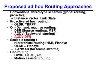
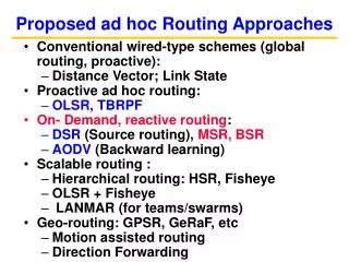
Proposed ad hoc Routing Approaches. Conventional wired-type schemes (global routing, proactive): Distance Vector; Link State Proactive ad hoc routing: OLSR, TBRPF On- Demand, reactive routing: DSR (Source routing), MSR AODV (Backward learning) Scalable routing :

E N D
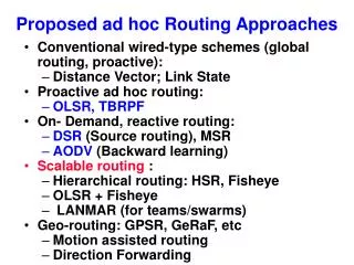
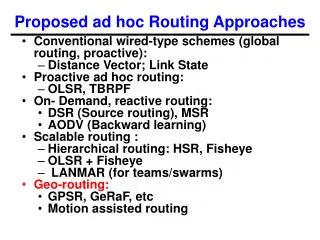
Proposed ad hoc Routing Approaches • Conventional wired-type schemes (global routing, proactive): • Distance Vector; Link State • Proactive ad hoc routing: • OLSR, TBRPF • On- Demand, reactive routing: • DSR (Source routing), MSR • AODV (Backward learning) • Scalable routing : • Hierarchical routing: HSR, Fisheye • OLSR + Fisheye • LANMAR (for teams/swarms) • Geo-routing: • GPSR, GeRaF, etc • Motion assisted routing
Georouting - Key Idea • Each node knows its geo-coordinates (eg, from GPS or Galileo) • Source knows destination geo-coordinates; it stamps them in the packet • Geo-forwarding: at each hop, the packet is forwarded to the neighbor closest to destination • Options: • Each node keeps track of neighbor coordinates • Nodes know nothing about neighbor coordinates
Closest to D A Geographic Routing: Greedy Routing S D • Find neighbors who are the closer to the destination • Forward the packet to the neighbor closest to the destination
Greedy Perimeter Stateless Routing for Wireless Networks (GPSR)– key elements • Greedy forwarding • Each nodes knows own coordinates • Source knows coordinates of destination • Greedy choice – “select” the most forward node
Greedy Forwarding does NOT always work • If the network is dense enough that each interior node has a neighbor in every 2/3 angular sector, GF will always succeed GF fails
Got stuck? Perimeter forwarding> Greedy forwarding failure. x is a local maximum in its geographic proximity to D; w and y are farther from D.> Node x’s void with respect to destination D
Greedy Perimeter Forwarding D is the destination; x is the node where the packet enters perimeter mode; forwarding hops are solid arrows;
TCP over GPSR, AODV, DSR and DSDV Throughput (Kbps) Speed(m/s)
GPSR commentary • Very scalable: • small per-node routing state • small routing protocol message complexity • robust packet delivery on densely deployed, mobile wireless networks • TCP is extremely sensitive to path breakage (timeout) -- It does very well with georouting • Outperforms DSR and AODV • Drawback: it requires knowledge of dest geo coordinates (explicit forwarding node address) • Beaconing overhead • nodes may go to sleep (on and off) in sensor networks
Energy-Aware geographic routing protocols in ad hoc networks
Next-hop selection in geographic routing • Different metrics determine different performance c d s b a
Next-hop selection in geographic routing • Select a node so that is minimized. Here p stands for power. k v a q m
Next-hop selection in geographic routing • 1. w is selected as anchor node. • 2. find a least cost path from u to w.
Geo Location Service Yinzhe Yu, et al : Enhancing Location Service Scalability With HIGH-GRADE , MASS 2004, Oct 2004
Position-Based Routing • Assuming each nodes is aware of its own geographical “location” and those of its neighbors • Forwarding packets based on destination location, using simple greedy forwarding and recovery strategies (Face2, GPSR)
Basic Problem For a node B wishing to communicate with another node A, how to discover current location of A? • How does A choose a set of nodes as its location servers, and how to update these servers as A moves around? (Location Server Organization) • What exact information about A’s location are stored on its location servers? (Location Information Granularity) • How does B find appropriate server(s) of A to obtain its location?
What is a Location Service? • A pre-requisite of Position-Based Routing is a Location Service • Allows a source node to obtain the location of a destination before data traffic follows • Location Service is a cooperative service • Each node in the MANET stores the current locations of some other nodes in the network, serving as their location server • A node updates its location servers as it moves around • A node trying to communicate with another node queries that node’s location servers to get its current location
B A Location Server Organization A B A B Flat structure: SLURP – Woo and Singh, 2001. Two-level structure: SLALoM – Cheng et al. 2002. DLM – Xue et al. 2002. Multi-level Hierarchical: GLS – Li et al., 2001.
Proposed : HIGH-GRADE • HIerarchicalGeographicalHash with multi-GRainedAddressDElegation • A better scheme that incorporates good design choices, and provides better scalability • Possible application: geo-routing in the urban vehicular grid
HIGH-GRADE divides a network area recursively into levels of “squares”. Each node chooses location servers around some hash points, one in each level of square. Each location server stores the information of “which next level square does A resides in ?”. A HIGH-GRADE Location Update
Location Info at Hash Points E G F D H C When there is no node at the exact location of the hash point, the update packet travels around the “perimeter” of the hash point and the location information is stored on all nodes on the perimeter.
B HIGH-GRADE Location Query • A querying node B uses the same hash functions to try potential location servers • Once a location server is found, it follows a series of servers at smaller and smaller area to pin-point A’s location • The total distance traveled by a location query message is proportional to the side length of A and B’s least common square A
Analysis: Model assumption • A common set of assumptions to analyze costs of maintaining and using a location service • A network with N nodes in an area of A • constant node density . • Average progress towards the destination point in each packet forwarding step is z. • Simplified random way-point mobility model with no pause time. Average node speed is v.
Metrics • Location Update Cost • Number of forwarding operations each node needs to perform in a second to handle the location update packets. • Location Query Cost • Number of forwarding operations each node needs to perform in a second to handle the location queries. • Storage Cost • Number of location records a node needs to store as a location server.
Summary of Results • Observations: • Design of a location service involves tradeoffs among all three metrics. • Not all schemes exploit the benefits of a localized traffic equally well. • For localized traffic HIGH-GRADE achieves impressive asymptotic scalability.
Simulation • Compare GLS and HIGH-GRADE • Confirm analytical results • ns2 with CMU Monarch extensions • N = 100 ~ 600 • Node density fixed at 100/km2 • Transmission range is 250 m • Mobility model: random waypoint (w/o pause) • Maximum speed 10~30 m/s • Load • Each node generates 15 location queries for random destination nodes during a 300 sec simulation time
A High-Throughput Path Metric for Multi-Hop Wireless Routing D. S. J. D. Couto, D. Aguayo, J. Bicket, and R. Morris. A High- Throughput Path Metric for Multi-Hop Wireless Routing. In Proceedings of ACM MobiCom, 2003.
Background • The most commonly used metric is minimum hop-count. • Links in route share radio spectrum • Extra hops reduce throughput Throughput = 1 Throughput = 1/2 Throughput = 1/3
Hop-count alone is insufficient Minimize hop-count B Delivery ratio = 100% 100% C A 20% If algorithm ignoring loss sees A>C as a link, it’ll choose A>C instead of A>B>C. Trade-off between hops and distance (Thus lossiness)- need to account for delivery rate in routing.
A test • A test was setup to see how the minimum hop count metric REALLY works. Note this was an experimental test, not a simulation. • During the test each packet sent contained 193 bytes (134 of data) • A “best” route was determined by trying 10 different routes and seeing which was best.
Indoor wireless network 29 PCs with 802.11b radios (fixed transmit power) in ‘ad hoc’ mode 2nd floor 3rd floor 5th floor 4th floor 6th floor
Testbed UDP throughput • The values above 225 correspond to pairs that communicated along single-hop paths; • those at or below 225 correspond to multi-hop paths. above 225 pkts/ s below 225 pkts /s
Results of the Test 2 hops 4 hops • 2 Regions • Above 250 PPS: 1 hop links • Below 250 PPS: Multihop links • Note the 0 values for 1/5 of the packets, even though a route exists 3 hops above 225 pkts/ s below 225 pkts /s
What throughput is possible? Routing protocol • when routing multi-hop, there is some throughput reduction to be expected • For one-hop routes, we get approximately as good as we deserve • For the rest of the multi-hop routes, DSDV still finds routes with much lower throughput than is possible ‘Best’
The shortest path does not yield the highest throughput Paths from 23 to 36 selects randomly from the shortest hopcount routes is unlikely to make the best choice
‘Good’ ‘Bad’ Challenge: many links are lossy One-hop broadcast delivery ratios Smooth link distribution complicates link classification.
Challenge: many links are asymmetric Broadcast delivery ratios in both link directions. Very asymmetric link. Many links are good in one direction, but lossy in the other.
New metric: ETX Minimize total transmissions per packet (ETX, ‘Expected Transmission Count’) Link throughput 1/ Link ETX Delivery Ratio Link ETX Throughput 100% 100% 1 50% 50% 2 33% 33% 3
Calculating ETX • Assuming 802.11 link-layer acknowledgments (ACKs) and retransmissions: • P(TX success) = P(Data success) P(ACK success) measured fwd delivery ratio rfwd measured rev delivery ratio rrev • Link ETX = 1 / P(TX success) = 1 / [ P(Data success) P(ACK success) ] • Link ETX 1 / (rfwd rrev) • Why measure both ACK and Data Success?
Route ETX Route ETX = Sum of link ETXs Route ETX Throughput 1 100% 2 50% 2 50% 3 33% 5 20%
Measuring Delivery Ratios • Each node broadcasts small link probes (134 bytes), once per second • Nodes remember probes received over past 10 seconds • Reverse delivery ratios estimated as rrev pkts received / pkts sent • Forward delivery ratios obtained from neighbors (piggybacked on probes)
DSDV overhead ETX improves DSDV throughput DSDV+hop-count better DSDV+ETX ‘Best’
DSR with ETX DSR+hop-count DSR+ETX ‘Best’
Summary • ETX is a new route metric for multi-hop wireless networks • ETX accounts for • Throughput reduction of extra hops • Lossy and asymmetric links • Link-layer acknowledgements • ETX finds better routes!