Electromagnetic compatibility in electrical power installations
240 likes | 457 Vues
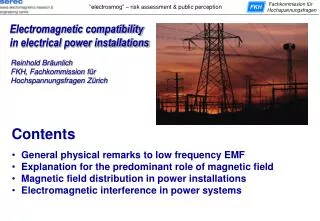
Electromagnetic compatibility in electrical power installations. Reinhold Bräunlich FKH, Fachkommission für Hochspannungsfragen Zürich. Contents. General physical remarks to low frequency EMF Explanation for the predominant role of magnetic field

Electromagnetic compatibility in electrical power installations
E N D
Presentation Transcript
Electromagnetic compatibilityin electrical power installations Reinhold BräunlichFKH, Fachkommission fürHochspannungsfragen Zürich Contents • General physical remarks to low frequency EMF • Explanation for the predominant role of magnetic field • Magnetic field distribution in power installations • Electromagnetic interference in power systems
Wavelength Frequency Hz Denotation Ionizing radiation Low frequency fields High frequency fields Infrared Biol.effects Force Nerve stimulus Heat Photo chemistry Ionization Abbrev. Terrestrialmagnetic field Lighting X-ray therapy Microwave Electricappliances Diathermy Sferics Laser applications Tramway Source Screen display X-ray radiography Power grid Infrared Lamp UHF RADAR Subway Radioactivity Sunlamp Railway Cellular phone Radio broadcast Atmospheric field Induction stove TV Satellite telecommunications
force force B field = E field = charge x velocity charge Newton Volt Unit: [Ns/Cm], [Vs/m2], [T] Unit: [N/C] or [V/m] Coulomb meter H field Ampère per meter [A/m]
Lorentz force Magnetic v Electric field Force u flux density ) ( q v F = E + x B FL Fq Charge 1 ( ) u x E = B with c2-u2 c· v2 ! verysmall ~ ~ q E FL = v = u then If c2
E fieldAppr. 850 1021 conduction electrons per meter: charge ~135 kC/mField strength if all conduction electrons are transfered: ~1.5x10¹⁸ V/mTheoretical force to the conductor: ~200x1021 NLimit of insulation: ~2.4x10⁶ V/m (factor of 1.57x10⁻¹²)Maximum realistic force to the conductor: ~0.51 N/m (factor of 2.46x10⁻²⁴) 1 cm + I 1 cm U, E 1 cm - I 1 cm F B F B field300 A are possible (electron velocity : 2.2 x 10⁻⁴ m/s)Magnetic flux density: 3x10⁻³ TForce: ~0.9 N/mTechnical flux densities ~1TResulting force to the conductor: ~300 N/m (factor of 330 compared to E field)
Properties Magnetic flux density B Electric field E Current in conductors Origin Charges normally at (conducting) surfaces Dependent on Operating current Operating voltage Effect in conductors (and biologic tissue) Eddy currents Displacement current Exiguous (by highly conducting materials) Influence by the environment Distorted by objects Penetrates in buildings Does not penetrate in stonewall buildings Penetration in buildings Lorentz force, Magnetostatic force Electrostatic force Action of force
d = p × × s × m × m 1 f 0 r Interaction of E and B field with matter „Shielding“ ØMaterials and electric field s > w × e × e Conductivity: 0 r e for 50 in materials with =1: Example: Hz r s r < W - 9 360 i.e. M m > × × p × × 50 2 8.854 2.79 10 A/Vm = S/m ØMaterials and the magnetic field Skin depth: For 50 Hz -> Copper: 9.4 mm,Aluminium: 12.3 mm,Iron (mr=200): 1.8 mm. Example: • To shielding mecanisms: • Guiding of the field in ferromagnetic material • Generation of a counter field by eddy currents in high conductive material
Display of vectors and phasors of two three-phase transmission systems L1 L3 L2 L2 L1 L3 Definition of window for the vector/phasor image
Wire 1 0.9 0.8 1/r 0.7 Flux density 0.6 0.5 0.4 0.3 0.2 0.1 0 0 1 2 3 4 5 6 7 8 9 10 r 2 or 3 phases 1/r2 Flux density r Loop 1/r3 Flux density = + + 2 2 2 d ( d d d ) / 2 1 2 3 r Characteristics of the decay of themagnetic flux density Single conductor Two-phase line Three-phase line 2-dimensional dipole field d: phase distance Loop, winding, apparatus 3-dimensional dipole field Orthogonal to the loop area: A: loop area
1.E+08 1.E+07 1.E+06 1.E+05 1.E+04 1.E+03 1.E+02 1.E+01 1.E+00 1.E-01 1.E-02 1.E-03 1.E-04 0.1 1 10 100 1000 Position [m] Characteristics of the decay of themagnetic flux density Phase current: 1000 A Decay with 1. power Decay with 2. power mT] Decay with 3. power Magnetic flux density [
1.E+08 Phase current: 1000 A Decay with 1. power 1.E+07 Decay with 2. power 1.E+06 Decay with 3. power mT] 1.E+05 Total expression 1.E+04 Exact calculation 1.E+03 1.E+02 Magnetic flux density [ 1.E+01 1.E+00 1.E-01 1.E-02 1.E-03 1.E-04 0.1 1 10 100 1000 Position [m] Characteristics of the decay of themagnetic flux density three-phase bus bar
Model for the magnetic flux decay of a transformer Worst-case value P : Nominal power of transformer kVA N k : Suggested proportionality constant 0.04 Tm3/kVA Tr r Distance of observer to the transformer centre m :
Calculated lines of constant RMS valueof the magnetic flux density • Transformer station 630 kVA, 16/0.4 kV, secondary current: 909 A • Program 1 • Program 2 By courtesy of:
a Lightning stroke in an earth wire Interference by athree-phasetransmission lineby earth fault with reversal breakdown resulting in a single-phase earth fault Earth wire I F2 I F3 I F 1 Phase conductors Voltage per E Length of pipeline u Pipeline Local potential difference
High frequency interference by switching transients Horizontal time scale: 5 ms/div Upper trace: cable charging current: 500 A/divLower trace: signal in secondary cable: 10 V/div Vertical:
Summary • Electric and magnetic fields are the responsible carrier for the electrical energy transportation • For the conversion of mechanical to electrical energy and vice versa the magnetic forces are used • For low frequency interference the magnetic field is much more significant than the electric field • The field distribution around electrical installationscan be described by simple expressions • In power systems low frequency and high frequency interference occur