Structural Equation Modeling
Structural Equation Modeling. Mgmt 290 Lecture 7 E xplanation of LISREL Results & E valuation of Models Nov. 9, 2009. Normal Distributions Assumptions Used. More on LISREL ML Estimation. # endogenous. To minimize Log| Σ(Θ)|+tr(S Σ -1 (Θ)) – log|S| -(p+q). F ml. # exogenous.

Structural Equation Modeling
E N D
Presentation Transcript
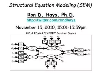
Structural Equation Modeling Mgmt 290 Lecture 7 Explanation of LISREL Results & Evaluation of Models Nov. 9, 2009
Normal Distributions Assumptions Used More on LISRELML Estimation # endogenous To minimize Log|Σ(Θ)|+tr(S Σ-1(Θ)) – log|S| -(p+q) Fml # exogenous tr --- sum of diagonal elements Σ(Θ)| -- model implied matrix S – observed matrix Fml =0 if Σ = S
Partial derivatives Algebraic solution Iterative • Starting values • - prior research, OLS results, LISREL automatic (by IV & 2SLS) • Methods to proceed • partial derivative of Fml of Θ • Final conversion Θ1, Θ2, Θ3 … , Θl
RC The ridge constant. This constant will be multiplied repeatedly by 10 until the matrix becomes positive-definite. Default: RC=0.001 More on toSpecify Outputs (1) • OU ME = IV/TS/UL/GL/ML/WL/DW RC=c NS NS If this option appears, the program will not compute starting values. The user must supply starting values with ST or MA commands. IV Instrumental variables TS Two-stage least squares UL Unweighted least squares GL Generalized least squares ML Maximum likelihoodWL Generally weighted least squares DW Diagonally weighted least squares
More on toSpecify Outputs (2) St Dev T Values Residuals Modification Indices Total Indirect • OU • SE TV RS EF MI ALL • Get more outputs • OU matrix1 = matrix2 = ... • save matrix • OU TM=t IT=n LY, LX, BE, GA, PH, PS, TE, TD TM The maximum number of CPU seconds for the current problem. Default: PC version, TM=172800 (2 days); IT Maximum number of iterations for the current problem. Default: IT=ten times the number of free parameters
Explanation of LISREL Results (1) Outputs for Path Analysis • Path coefficients • Hypothesis testing results
Equation Coefficients LISREL Estimates (Maximum Likelihood) • Structural Equations • Y1 = - 0.087*X2, Errorvar.= 12.96, R² = 0.11 • (0.019) (1.41) • -4.65 9.22 • Y2 = - 0.28*Y1 + 0.058*X2, Errorvar.= 8.49 , R² = 0.23 • (0.062) (0.016) (0.92) • -4.58 3.59 9.22 • Y3 = - 0.22*Y1 + 0.85*Y2 + 0.86*X1, Errorvar.= 19.45, R² = 0.39 • (0.098) (0.11) (0.34) (2.11) • -2.23 7.53 2.52 9.22 Ex3a.spl Sample size < 120 Use T table Otherwise, use Z table
Total & Indirect Effects Use OU EF See Ex3aef.ls8 • Total Effects of Y on Y • Y1 Y2 Y3 • -------- -------- -------- • Y1 - - - - - - • Y2 -0.28 - - - - • (0.06) • -4.58 • Y3 -0.46 0.85 - - • (0.10) (0.11) • -4.41 7.53 OR LISREL OUTPUT: EF In SIMPLIS
Explanation of LISREL Results (2) Output for CFA • Loadings • Error variances • R 2
Ex5a.spl Loadings and R2 • VIS PERC = 0.672*Visual, Errorvar.= 0.548 , R² = 0.452 • (0.0910) (0.0971) • 7.388 5.645 • CUBES = 0.513*Visual, Errorvar.= 0.737 , R² = 0.263 • (0.0924) (0.101) • 5.551 7.300 • LOZENGES = 0.684*Visual, Errorvar.= 0.532 , R² = 0.468 • (0.0910) (0.0974) • 7.516 5.461 • PAR COMP = 0.867*Verbal, Errorvar.= 0.248 , R² = 0.752 • (0.0702) (0.0515) • 12.348 4.819 • ……
Explanation of LISREL Results (3) Hybrid Model Outputs • A combination of • Path coefficients • Loadings
Path Coefficients & Loadings LISREL Estimates (Maximum Likelihood) • Measurement Equations • ANOMIA67 = 2.66*Alien67, Errorvar.= 4.74 , R² = 0.60 • (0.45) • 10.43 • … • Error Covariance for ANOMIA71 and ANOMIA67 = 1.62 • (0.31) • 5.17 • … • Structural Equations • Alien67 = - 0.56*Ses, Errorvar.= 0.68 , R² = 0.32 • (0.047) (0.066) • -12.09 10.35 • Alien71 = 0.57*Alien67 - 0.21*Ses, Errorvar.= 0.50 , R² = 0.50 • (0.048) (0.046) (0.050) • 11.89 -4.52 10.10
Explanation of LISREL Results (4) Fit Indices • Chi-square • Chi-square / df < 3 Compare to just-identified (N-1)Fml Σ vs. Σ(θ) Increases as N Not good for large sample
Relative amount of the variance In S that are predicted by Σ Fit Indices • GFI • AGFI • NFI= 1-F/Fi • CFI • NNFI GFI = 1 – tr[(Σ-1 S- I)2] / tr[(Σ-1 S) 2 AGFI = 1 – [q(q+1)/2 df] [ 1-GFI] Close to 1 Compare to a baseline model
Fit Indices • RMR • Root Mean squared Residual • SRMR – Standardized Root Mean Squared Residual • RMSEA – Root Mean Square Error of Approximation RMR=[2 ΣΣ(sij-δij)2 / q(q+1)] 1/2 Close to 0
Parsimonious Fit • AIC • CAIC • PNFI=dfmodel/dfindep X NFI • PGFI=1-(P/N)GFI Chi-square adjusted for df - 2df
Relative Fit • NFI, NNFI – compare to indep model • Compare nested model • use Chi-square difference
Common Practice in Reporting- 3 must-report items • Chi-square, DF, Significance • GFI or NFI or CFI • NNFI or AGFI • SRMR
What is considered as a good fit • Chi-square/df <3 • GFI >.95 • SRMR <.08 • And check residuals
Modification Indexes • Each such modification index measures how much chi-square is expected to decrease if this particular parameter is set free and the model is re-estimated. • (Comparative fit for ONE parameter)
3 Foundation for Model Re-specification • Theory-based revisions • Modification Indices • Residual Matrix
ExampleSIMPLIS The Modification Indices Suggest to Add the Path to from Decrease in Chi-Square New Estimate x1 dem 13.7 -5.83 x4 dem 26.3 7.93 x5 lib 119.9 41.83 x8 lib 9.4 -5.88 The Modification Indices Suggest to Add an Error Covariance Between and Decrease in Chi-Square New Estimate x2 x1 19.8 1.42 x4 x3 11.1 -0.63 x5 x3 18.0 0.51 x6 x3 13.4 -0.82 x6 x4 11.2 1.28 x6 x5 9.7 -0.74 x7 x3 8.1 -0.85 x7 x6 42.5 4.41 x8 x4 14.8 1.11 x8 x6 78.9 3.27 x8 x7 16.2 2.01 • Bollen80.spl • Bollen80n.spl
Example for LISREL Expected Change for LAMBDA-X pollib demo -------- -------- x1 - - -5.83 x2 - - -4.20 x3 - - 1.27 x4 - - 7.93 x5 41.83 - - x6 -5.24 - - x7 -4.61 - - x8 -5.88 - - • Bollen80.ls8 • Use MI in OU
Two Roads to Parsimonious Model (1) Model Trimming • Delete links to achieve a parsimonious model • Start from the most complicated model To get a parsimonious model
(2) Model Building • Add links to build a better model • You may start from the simplest model • and move up To get a model of good fit