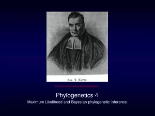
Phylogenetics 4 Maximum Likelihood and Bayesian phylogenetic inference
http://www.york.ac.uk/depts/maths/histstat/people/. Phylogenetics 4 Maximum Likelihood and Bayesian phylogenetic inference . Previously: The parsimony criterion Bootstrapping Models of molecular evolution Distance methods

Phylogenetics 4 Maximum Likelihood and Bayesian phylogenetic inference
E N D
Presentation Transcript
http://www.york.ac.uk/depts/maths/histstat/people/ Phylogenetics 4 Maximum Likelihood and Bayesian phylogenetic inference
Previously: The parsimony criterion Bootstrapping Models of molecular evolution Distance methods Model-based distance corrections for distance analyses (e.g., Fitch-Margoliash, Neighbor-Joining, UPGMA) Today: The likelihood criterion More on models of molecular evolution Maximum likelihood analysis Performance of distance, parsimony, and ML analyses in simulation (Huelsenbeck, 1995) Bayesian phylogenetic inference
Parsimony criterion: The “shortest” tree is optimal. Tree length is dependent on the step matrix for transformation costs. Pros: Intuitive Analytically tractable Flexible--many different weighting schemes possible Can combine different kinds of data
Parsimony criterion: The “shortest” tree is optimal. Tree length is dependent on the step matrix for transformation costs. Cons: May be inconsistent in the statistical sense, meaning that as more and more data are accumulated, results can converge on an incorrect solution. Consider tree with a short internal branch and asymmetric terminal branches, reflecting unequal rates of evolution. Using parsimony, correct reconstruction of the internal branch requires a character that changed along the internal branch, but not on terminal branches. It is unlikely that such informative characters will occur, but uninformative or misinformative characters may be common. Parsimony can be "positively misleading" in cases like these, because the number of misinformative characters will increase as the number of characters increases. So, parsimony will cause you to become more confident in the wrong answer. This tree scenario has been called the "Felsenstein zone”. The phylogenetic artifact is called long branch attraction. http://www.gs.washington.edu/faculty/images/felsenstein.jpg Swofford et al p. 427 fig. 8
The likelihood criterion: The tree that maximizes the likelihood of the observed data is optimal. L = P(datatree, model) Likelihood (L) is the probability of the data (alignment), given a tree (with topology and branch lengths specified) and a probabilistic model of evolution. Assumptions (the fine print): The tree is correct The probability that a position has a certain state at time 1 depends only on the state at time 0; knowing that it had some state prior to time 0 is irrelevant--this is called a Markov process Data (individual sites) are independent A uniform evolutionary process operated across the entire tree (why might this be false? endosymbiosis? loss of function?), i.e., the process of evolution is a homogeneous Markov process. Maximum likelihood methods are explicitly model-based. Examples of models….
Two simple models of molecular evolution: Jukes-Cantor (JC69) one-parameter model Assumes that all transformations between nucleotides occur at the same rate Kimura (K80 or K2P) two-parameter model Assumes that transitions and transversions occur at different rates (supported by empirical data). AC AC Transitions Transversions GT GT K2P JC69
Models of molecular evolution are based on substitution rate matrices (and which can be transformed into substitution probability matrices). Models vary in the numbers and kinds of parameters used to determine elements in the rate matrix JC69* rate matrix 1 parameter: a “To” state “From” state *Jukes, T. H., and C. R. Cantor. 1969. Evolution of protein molecules. Pages 21-132 in H. N. Munro (ed.), Mammalian Protein Metabolism. Academic Press, New York. © Paul Lewis
K80* (or K2P) rate matrix 2 parameters: a b “To” state rate of transversions is b rate of transitions is a “From” state The diagonal elements make rows sum to 0 *Kimura, M. 1980. A simple method for estimating evolutionary rate of base substitutions through comparative studies of nucleotide sequences. Journal of Molecular Evolution 16:111-120. © Paul Lewis
Felsenstein 1981 (F81) model: Transformation rates determined by mean substitution rate (m) and equilibrium base frequencies (e.g., pA) 4 parameters: pA pC pG m Identical to the JC69 model if all the base frequencies are set to ¼. *Felsenstein, J. 1981. Evolutionary trees from DNA sequences: a maximum likelihood approach. Journal of Molecular Evolution 17:368-376. © Paul Lewis
Hasegawa-Kishino-Yano 1985 (HKY85) model: Transformation rates determined by mean substitution rate (b), transition-transversion rate ratio (k) and equilibrium base frequencies (e.g., pA) 5 parameters: pA pC pG k b Identical to the F81 model if k = 1. Identical to the JC69 model if k = 1 and all the base frequencies are set to ¼. *Hasegawa, M., H. Kishino, and T. Yano. 1985. Dating of the human-ape splitting by a molecular clock of mitochondrial DNA. Journal of Molecular Evolution 21:160-174. © Paul Lewis
Generalized time reversible (GTR) model: Transformation rates determined by mean substitution rate (m), relative rate parameters (a-e) and base frequencies (e.g., pA) 9 parameters: pA pC pG a b c d e m -m (pAc + pCe + pGf) Identical to the JC69 model if a = b = c = d = e = f = 1 and all the base frequencies are set to ¼. *Lanave, C., G. Preparata, C. Saccone, and G. Serio. 1984. A new method for calculating evolutionary substitution rates. Journal of Molecular Evolution 20:86-93. © Paul Lewis
The models discussed so far are interconvertible by adding or restricting parameters. Swofford et al. p. 434
Elaborations to GTR (and other nucleotide models): Modifications to accommodate rate heterogeneity Discrete gamma () model of rate heterogeneity (rates of evolution for each site are distributed according to a “discretized” gamma distribution) Proportion of invariant (I) sites model (some sites assumed to be invariant) Combinations of the above, e.g., GTR + + I model Molecular clock models Strict clock models (uniform rates of evolution across the phylogeny) Relaxed clock models (rates allowed to vary across branches) Correlated relaxed clock (rates of adjacent branches are correlated) Uncorrelated relaxed clock (rates of adjacent branches are independent) Other kinds of models used in phylogenetics: Amino acid sequence models: Dayhoff; PAM; Wagner, etc Codon-based nucleotide models Morphological character models Correlated (nonindependent) models for morphological or molecular characters Various methods exist for choosing models of molecular evolution (aiming for a model that is not underparameterized [poor fit to observed data] or overparameterized [poor predictive power; computationally intensive]). Criteria: Likelihood ratio test; Akaike Information Criterion (AIC); Bayesian Information Criterion (BIC) Programs by David Posada and colleagues: Modeltest (nucleotides)http://darwin.uvigo.es/software/modeltest.html, ProtTest (amino acids)http://darwin.uvigo.es/software/prottest.html
Calculating the likelihood of a tree. • L = P(datatree, model) • Consider a tree, with four species and branch lengths specified, and an aligned dataset • For each site, there are four observed tip states and sixteen (4x4) possible combinations of ancestral states • Each reconstruction of ancestral states has a probability, based on the transformation probability matrix and branch lengths • The likelihood of the tree for the one site is equal to the sum of the probabilities of each reconstruction of ancestral states • The likelihood of the entire dataset given the tree is the product of the likelihoods of the individual sites, or the sum of the log likelihoods of the sites • This calculation is repeated on multiple trees, and the tree that provides the highest likelihood score is preferred. The process of generating the trees can use exhaustive, branch-and-bound, or heuristic searches (often with starting trees generated with parsimony or distance searches). Graur and Li Fig 5.19
Likelihood caluculations, continued.Brute force approach would be to calculate Lfor all 16 combinations of ancestral states and sum © Paul Lewis
Pruning algorithm* (same result, much less time) Many calculations can be done just once, and then reused many times *The pruning algorithm was introduced by: Felsenstein, J. 1981. Evolutionary trees from DNA sequences: a maximum likelihood approach. Journal of Molecular Evolution17:368-376 © Paul Lewis
Recent algorithms have dramatically improved the efficiency of ML calculations. e.g., RAxML by Alexi Stamatakis http://icwww.epfl.ch/~stamatak/index.htm GARLI by Derrick Zwickl http://www.bio.utexas.edu/faculty/antisense/garli/Garli.html Nonetheless, ML calculations are still a lot of work. Are they worth it? John Huelsenbeck performed a classic, and still relevant, study to test accuracy of parsimony, ML, and distance methods (Huelsenbeck, J. 1995. Performance of phylogenetic methods in simulation. Syst. Biol. 44: 17-48) • Simulations: • 4-taxon trees with varying branch lengths (including the Felsenstein zone) implying change in 1% to 75%; total of 1296 (parsimony, distance) or 676 (ML) combinations of branch lengths. • Datasets “evolved” on each tree under three models: Jukes-Cantor, Kimura 2-parameter (with 5:1 transition/transversion bias), JC with among-site rate heterogeneity • 1000 simulated datasets were produced for each of 1296 trees; except ML, with 100 datasets for each of 676 trees • Phylogenetic analyses were performed for each tree/dataset combination using 26 analytical methods, with 100, 500, 1000, 10000 or infinite sites.
Results: • Results for simple parsimony on data generated under Jukes-Cantor model. • 95% isocline indicates region within which the correct tree is estimated 95% of the time. • Increasing data improves accuracy, up to a point--in the Felsenstein zone, even infinite data do not allow correct reconstruction of the phylogeny. Parsimony is inconsistent.
Results continued: • Results for 26 methods on data generated under Jukes-Cantor model. • Black: correct tree is recovered 100% of the time. White: correct tree never recovered. Gray: intermediate. • White lines: 95% isocline (region within which the correct tree is estimated 95% of the time). • Black lines: 33% isocline (equivalent to picking a tree at random).
What does it mean?: For all methods, more data are better, but… • Parsimony is inconsistent, even when character-state weighting is applied. • Model-based distance corrections improve performance of minimum evolution distance method • UPGMA performs poorly, perhaps due to implicit assumption of equal rate of evolution • ML performs best, but still has trouble in the FZ
ML appears to be an accurate method under a wide range of treespace (and modelspace). But… ML is still computationally intensive. Intuitively the Likelihood of the data L = P(datatree, model) is not really what we care about. (After all, we have observed the data.) What we really want to know is, what is the probability of the tree: P(treedata) Bayes’ theorem allows estimation of the posterior probability of a tree, given a prior probability (marginal probability) of the tree. 1702-1761
Bayes' rule in Statistics D refers to the "observables" (i.e. the Data) q refers to one or more "unobservables" (i.e. parameters of a model, or the modelitself): • tree model (i.e. tree topology) • substitution model (e.g. JC, F84, GTR, etc.) • parameter of a substitution model (e.g. a branch length, a base frequency, transition/transversion rate ratio, etc.) • hypothesis (i.e. a special case of a model) © Paul Lewis
Bayes' rule in Statistics Likelihood of hypothesis q Prior probability of hypothesis q Posterior probability of hypothesis q Marginal probability of the data (marginalizing over hypotheses) © Paul Lewis
Bayesian estimation Example using dice from the manual for MrBayes, the standard program for Bayesian phylogenetic analysis, by Frederik Ronquist and John Huelsenbeck http://mrbayes.csit.fsu.edu/
Bayesian estimation in phylogenetics • Calculating the posterior probability of the tree • Given a tree, aligned data, prior probability of tree • Note that the likelihood f(tX) is integrated over all possible values of branch lengths and parameter values--means that the posterior probability takes account of all possible topologies, branch lengths and substitution parameters • Denominator is a summation of the likelihood of a tree times the prior probability of the tree over all trees • All trees are considered equally likely a priori--in other words, the prior probabilities are said to be "flat" or "uniform” • Consequently, the posterior probability of a tree cannot be calculated! • Fortunately, Markov chain Monte Carlo (MCMC) simulation can be used to sample the posterior probability distribution
Bayesian estimation in phylogenetics • MCMC simulation • Begin with a model (tree and model parameters) and estimate the likelihood • Perturb the model--change the tree topology and branch lengths, and/or modify the parameter values • Determine whether the new model is accepted • If the new model has higher probability than the preceding model, the new state is accepted • If the new model has a lower probability than the preceding model, calculate the acceptance ratio • The greater the difference in probabilities of the new and old states, the greater the chance that it will be rejected] • MCMC differs from a heuristic search in that the "uphill" steps are automatically accepted, but the "downhill" steps are not automatically rejected • MCMC takes a random walk through treespace, but tends to remain in the area where the probability is most dense • continue for n generations • Eventually, a set of accepted models (trees plus substitution parameters) will be obtained, which is a sample from the posterior probability. • From this distribution, the posterior probabilities of all variable elements of the model can be estimated directly. • Calculate majority-rule tree; frequency of clade is its posterior probability, reported on interval 0.0-1.0 (vs. bootstrap frequencies, 0-100%)
MCMC robot’s rules Drastic “off the cliff” downhill steps are almost never accepted Slightly downhill steps are usually accepted With these rules, it is easy to see why the robot tends to stay near the tops of hills Uphill steps are always accepted © Paul Lewis
(Actual) MCMC robot rules Drastic “off the cliff” downhill steps are almost never accepted because R is near 0 10 Slightly downhill steps are usually accepted because R is near 1 8 Currently at 6.2 m Proposed at 5.7 m R = 5.7/6.2 =0.92 6 Currently at 6.2 m Proposed at 0.2 m R = 0.2/6.2 = 0.03 4 Currently at 1.0 m Proposed at 2.3 m R = 2.3/1.0 = 2.3 2 0 Uphill steps are always accepted because R > 1 The robot takes a step if it draws a Uniform(0,1) random deviate that is less than or equal to R © Paul Lewis
What MCRobot can teach us about Markov chain Monte Carlo • Posterior distribution: • equal mixture of 3 bivariate normal “hills” • inner contours: 50% • outer contours: 95% • Proposal scheme: • random direction • gamma-distributed step length • reflection at edges Here you are looking down from above at one of the three bivariate normal hills © Paul Lewis
Random walk In this case, the robot is accepting every step. 5000 steps are shown. The robot left a dot each place it stepped. Density of points does not reflect probability density (that is, a pure random walk does not help us) © Paul Lewis
Robot is now following the rules and thus quickly finds one of the three hills First 100 steps Note that first few steps are not at all representative of the distribution (this is the “burn-in” period) Starting point © Paul Lewis
Target distribution approximation 5000 steps taken • How good is the MCMC • approximation? • 51.2% of points are inside inner contours (cf. 50% actual) • 93.6% of points are inside outer contours (cf. 95% actual) • Approximation gets • better the longer the • chain is allowed to run. © Paul Lewis
Just how long is a long run? What would you conclude about the target distri- bution had you stopped the robot at this point? The way to avoid this mistake is to perform several runs, each one beginning from a different randomly-chosen starting point. Results different among runs? Probably none of them were long enough! 1000 steps taken © Paul Lewis
Moving through treespace The Larget-Simon* move *Larget, B., and D. L. Simon. 1999. Markov chain monte carlo algorithms for the Bayesian analysis of phylogenetic trees. Molecular Biology and Evolution 16: 750-759. See also: Holder et al. 2005. Syst. Biol. 54: 961-965. © Paul Lewis
Moving through parameter space Using k (ratio of the transition rate to the transversion rate) as an example of a model parameter. Proposal distribution is the uniform distribution on the interval (k-d, k+d) The “step size” of the MCMC robot is defined by d: a larger d means that the robot will attempt to make larger jumps on average. © Paul Lewis
History plots Burn-in is over right about here “White noise” appearance is a good sign L Important! This is a plot of first 1000 steps, and there is no indication that anything is wrong (but we know for a fact that we didn’t let this one run long enough) We started off at a very low point © Paul Lewis
Putting it all together • Start with random tree and arbitrary initialvalues for branch lengths and model parameters • Each generation consists of one of these (chosen at random): • Propose a new tree (e.g. Larget-Simon move) and either accept or reject the move • Propose (and either accept or reject) a new model parameter value • Every k generations, save tree, branch lengthsand all model parameters (i.e. sample the chain) • After n generations, summarize sample usinghistograms, means, credibility intervals, majority-rule consensus trees, etc. © Paul Lewis
Marginal Posterior Distribution of k Histogram created from a sample of 1000 kappa values. lower = 2.907 upper = 3.604 95% credible interval Lewis, L., and Flechtner, V. 2002. Taxon 51: 443-451. mean = 3.234 © Paul Lewis
Sources: Paul Lewis, Dept. of Ecology and Evolutionary Biology, University of Connecticut. EEB 349: Phylogenetics http://www.eeb.uconn.edu/people/plewis/index.php DL Swofford, GJ Olsen, PJ Waddell, DM Hillis. 1996. Phylogenetic Inference. Pp. 407-514 in DM Hillis, C Moritz, BK mable (eds.). Molecular Systematics 2nd Ed. Sinauer Assoc. D Graur, WH Li. 2000. Fundamentals of Molecular Evolution 2nd Ed. Sinauer Assoc. S Freeman, JC Herron. 2001. Evolutionary Analysis 2nd Ed. Prentice Hall. NA Campbell, JB Reece. 2005. Biology 7th Ed. Pearson.