LECTURE 07: MAXIMUM LIKELIHOOD AND BAYESIAN ESTIMATION
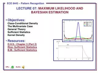
LECTURE 07: MAXIMUM LIKELIHOOD AND BAYESIAN ESTIMATION. • Objectives: Class-Conditional Density The Multivariate Case General Theory Sufficient Statistics Kernel Density Resources: D.H.S.: Chapter 3 (Part 2) Rice: Sufficient Statistics B.M.: Sufficient Statistics. Audio:. URL:.

LECTURE 07: MAXIMUM LIKELIHOOD AND BAYESIAN ESTIMATION
E N D
Presentation Transcript
LECTURE 07: MAXIMUM LIKELIHOOD ANDBAYESIAN ESTIMATION • Objectives:Class-Conditional DensityThe Multivariate CaseGeneral TheorySufficient StatisticsKernel Density • Resources:D.H.S.: Chapter 3 (Part 2)Rice: Sufficient StatisticsB.M.: Sufficient Statistics Audio: URL:
Introduction to Bayesian Parameter Estimation (Review) • In Chapter 2, we learned how to design an optimal classifier if we knew the prior probabilities, P(i), and class-conditional densities, p(x|i). • Bayes: treat the parameters as random variables having some known prior distribution. Observations of samples converts this to a posterior. • Bayesian learning: sharpen the a posteriori density causing it to peak near the true value. • Supervised vs. unsupervised: do we know the class assignments of the training data. • Bayesian estimation and ML estimation produce very similar results in many cases. • Reduces statistical inference (prior knowledge or beliefs about the world) to probabilities.
Class-Conditional Densities (Review) • Posterior probabilities, P(i|x), are central to Bayesian classification. • Bayes formula allows us to compute P(i|x) from the priors,P(i), and the likelihood, p(x|i). • But what If the priors and class-conditional densities are unknown? • The answer is that we can compute the posterior, P(i|x), using all of the information at our disposal (e.g., training data). • For a training set, D, Bayes formula becomes: • We assume priors are known: P(i|D) = P(i). • Also, assume functional independence:Di have no influence on • This gives:
Univariate Gaussian Case (Review) • p(|D) is an exponential of a quadratic function, which makes it a normal distribution. Because this is true for any n, it is referred to as a reproducing density. • p() is referred to as a conjugate prior. • Write p(|D) ~ N(n,n2): • and equate coefficients: • Two equations and two unknowns. Solve for n and n2:
Bayesian Learning (Review) • nrepresents our best guess after n samples. • n2represents our uncertainty about this guess. • n2approaches 2/n for large n – each additional observation decreases our uncertainty. • The posterior, p(|D), becomes more sharply peaked as n grows large. This is known as Bayesian learning.
Class-Conditional Density • How do we obtain p(x|D) (derivation is tedious): where: • Note that: • The conditional mean, n, is treated as the true mean. • p(x|D) and P(j) can be used to design the classifier.
Assume: • where are assumed to be known. Multivariate Case • Applying Bayes formula: which has the form: • Once again: and we have a reproducing density.
Equating coefficients between the two Gaussians: • The solution to these equations is: • It also follows that: Estimation Equations
General Theory • p(x| D) computation can be applied to any situation in which the unknown density can be parameterized. • The basic assumptions are: • The form of p(x| ) is assumed known, but the value of is not known exactly. • Our knowledge about is assumed to be contained in a known prior density p(). • The rest of our knowledge is contained in a set D of n random variables x1, x2, …, xndrawn independently according to the unknown probability density function p(x).
Formal Solution • The posterior is given by: • Using Bayes formula, we can write p(D| ) as: • and by the independence assumption: • This constitutes the formal solution to the problem because we have an expression for the probability of the data given the parameters. • This also illuminates the relation to the maximum likelihood estimate: • Supposep(D| ) reaches a sharp peak at .
Comparison to Maximum Likelihood • This also illuminates the relation to the maximum likelihood estimate: • Supposep(D| ) reaches a sharp peak at . • p(| D) will also peak at the same place if p() is well-behaved. • p(x|D) will be approximately , which is the ML result. • If the peak of p(D| ) is very sharp, then the influence of prior information on the uncertainty of the true value of can be ignored. • However, the Bayes solution tells us how to use all of the available information to compute the desired density p(x|D).
Recursive Bayes Incremental Learning • To indicate explicitly the dependence on the number of samples, let: • We can then write our expression for p(D| ): • where . • We can write the posterior density using a recursive relation: • where . • This is called the Recursive Bayes Incremental Learning because we have a method for incrementally updating our estimates.
When do ML and Bayesian Estimation Differ? • For infinite amounts of data, the solutions converge. However, limited data is always a problem. • If prior information is reliable, a Bayesian estimate can be superior. • Bayesian estimates for uniform priors are similar to an ML solution. • If p(| D) is broad or asymmetric around the true value, the approaches are likely to produce different solutions. • When designing a classifier using these techniques, there are three sources of error: • Bayes Error: the error due to overlapping distributions • Model Error: the error due to an incorrect model or incorrect assumption about the parametric form. • Estimation Error: the error arising from the fact that the parameters are estimated from a finite amount of data.
Noninformative Priors and Invariance • The information about the prior is based on the designer’s knowledge of the problem domain. • We expect the prior distributions to be “translation and scale invariance” – they should not depend on the actual value of the parameter. • A priorthat satisfies this property is referred to as a “noninformative prior”: • The Bayesian approach remains applicable even when little or no prior information is available. • Such situations can be handled by choosing a prior density giving equal weight to all possible values of θ. • Priors that seemingly impart no prior preference, the so-called noninformative priors, also arise when the prior is required to be invariant under certain transformations. • Frequently, the desire to treat all possible values of θ equitably leads to priors with infinite mass. Such noninformative priors are called improper priors.
Example of Noninformative Priors • For example, if we assume the prior distribution of a mean of a continuous random variable is independent of the choice of the origin, the only prior that could satisfy this is a uniform distribution (which isn’t possible). • Consider a parameter , and a transformation of this variable:new variable, . Suppose we also scale by a positive constant: . A noninformative prior on is the inverse distribution p() = 1/ , which is also improper.
Sufficient Statistics • Direct computation of p(D|) and p(|D)for large data sets is challenging(e.g. neural networks) • We need a parametric form for p(x|) (e.g., Gaussian) • Gaussian case: computation of the sample mean and covariance, which was straightforward, contained all the information relevant to estimating the unknown population mean and covariance. • This property exists for other distributions. • A sufficient statistic is a function s of the samples D that contains all the information relevant to a parameter, . • A statistic, s, is said to be sufficient for if p(D|s,) is independent of :
The Factorization Theorem • Theorem: A statistic, s, is sufficient for , if and only if p(D|) can be written as: . • There are many ways to formulate sufficient statistics(e.g., define a vector of the samples themselves). • Useful only when the function g() and the sufficient statistic are simple(e.g., sample mean calculation). • The factoring of p(D|) is not unique: • Define a kernel density invariant to scaling: • Significance: most practical applications of parameter estimation involve simple sufficient statistics and simple kernel densities.
Gaussian Distributions • This isolates the dependence in the first term, and hence, the sample mean is a sufficient statistic using the Factorization Theorem. • The kernel is:
The Exponential Family • This can be generalized: and: • Examples:
Summary • Bayesian estimates of the mean for the multivariate Gaussian case. • General theory for Bayesian estimation. • Comparison to maximum likelihood estimates. • Recursive Bayesian incremental learning. • Noninformative priors. • Sufficient statistics • Kernel density.