Motion Detail Preserving Optical Flow Estimation
840 likes | 1.11k Vues
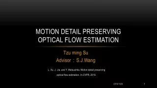
Motion Detail Preserving Optical Flow Estimation. Tzu ming Su Advisor : S.J.Wang. L. Xu , J. Jia , and Y. Matsushita. Motion detail preserving optical flow estimation. In CVPR, 2010. Outline. Previous Work Optical flow Conventional optical flow estimation. CCD. 3D motion vector.

Motion Detail Preserving Optical Flow Estimation
E N D
Presentation Transcript
Motion Detail Preserving Optical Flow Estimation Tzu ming Su Advisor:S.J.Wang L. Xu, J. Jia, and Y. Matsushita. Motion detail preserving optical flow estimation. In CVPR, 2010.
Outline • Previous Work • Optical flow • Conventional optical flow estimation
CCD 3D motion vector 2D optical flow vector Motion Field • Definition:anideal representation of 3D motion as it is projected onto a camera image.
Motion field • Applications: • Video enhancement:stabilization, denoising, super resolution • 3D reconstruction:structure from motion (SFM) • Video segmentation • Tracking/recognition • Advanced video editing (label propagation)
Motion field estimation • Optical flow Recover image motion at each pixel from spatio-temporal image brightness variations • Feature-tracking Extract visual features (corners, textured areas) and “track” them over multiple frames
Optical flow • Definition:the apparent motion of brightness patterns in the images • Map flow vector to color • Magnitude: saturation • Orientation: hue
Optical flow • Key assumptions • Brightness constancy • Small motion • Spatial coherence Remark:Brightness constancy is often violated • Use gradient constancy for addition, both of them are called data constraint
Ix v It Brightness consistency • 1-D case
Brightness consistency • 1-D case I ( x , t ) v ? p
Temporal derivative Spatial derivative Brightness consistency • 1-D case v I ( x , t ) p
Brightness consistency • 1-D case • 2-D case One equation, two velocity (u,v) unknowns… v u
Time t Time t+dt Aperture Problem • We know the movement parallel to the direction of gradient , but not the movement orthogonal to the gradient • We need additional constraints ?
Conventional estimation • Use data consistency & additional constraint to estimate optical flow • Horn-Schunck • Minimize energy function with smoothness term • Lucas-Kanade • Minimize least square error function with local region coherence
Horn-Schunck estimation • Imposing spatial smoothness to the flow field • Adjacent pixels should move together as much as possible • Horn & Schunckequation
Horn-Schunck estimation • Use 2D Euler Lagrange • Can be iteratively solved
Coarse to fine estimation • Optical flow is assumed to be small motions , but in fact most motions are not • Solved by coarse to fine resolution
run iteratively . . . image It-1 image I Coarse to fine estimation run iteratively
Outline • Previous Work • Contributions • Extended Flow Initialization • Selective data term • Efficient optimization solver • Experimental result • Conclusion
Outline • Previous Work • Contributions • Extended Flow Initialization • Selective data term • Efficient optimization solver • Experimental result • Conclusion
Muti-scale problem • Conventional coarse to fine estimation can’t deal with large displacement. • With different motion scales between foreground & background , even small motions can be miss detected.
Ground truth Ground truth Estimate Estimate Estimate … Ground truth
Muti-scale problem • Large discrepancy between initial values and optimal motion vectors • Solution: Improve flow initialization to reduce the reliance on the initializationfromcoarser levels
Selection Fusion Sparse feature matching Dense nearest-neighbor patch matching
Extended Flow Initialization • Sparse feature matching for each level
Extended Flow Initialization • Identify missing motion vectors
Extended Flow Initialization • Identify missing motion vectors
Extended Flow Initialization Fuse …
Selection Fusion Sparse feature matching Dense nearest-neighbor patch matching
Outline • Previous Work • Contributions • Extended Flow Initialization • Selective data term • Efficient optimization solver • Experimental result • Conclusion
constraints • Brightness consistency • Gradient consistency • Average
constraints • Pixels moving out of shadow • Color constancy is violated : ground truth motion of p1 • Gradient constancy holds • Average:
constraints • Pixels undergoing rotational motion • Color constancy holds : ground truth motion of p2 • Gradient constancy is violated • Average:
Selective data term • Selectively combine the constraints where
Selective data term selective
Outline • Previous Work • Contributions • Extended Flow Initialization • Selective data term • Efficient optimization solver • Experimental result • Conclusion
Discrete-optimization • Minimizing energy including discrete α & continuous u: • Try to separate α & u • For α • Probability of a particular state of MRF system
Discrete-optimization • Partition function • Sum over all possible values of α
Discrete-optimization • Optimal condition (Euler-Lagrange equations) • It decomposes to • Minimization • Update α • Compute flow field
continuous-optimization • Energy function • Variable splitting
continuous-optimization • Fix u , estimate w,p • Fix w,p , estimate u • The Euler-Lagrange equation Is linear.
Outline • Previous Work • Contributions • Extended Flow Initialization • Selective data term • Efficient optimization solver • Experimental result • Conclusion
selective data term Difference Selective Averaging
Results from Different Steps Coarse-to-fine Extended coarse-to-fine
Large Displacement Overlaid Input