Optical Flow Estimation using Variational Techniques
Optical Flow Estimation using Variational Techniques . Darya Frolova. Part I. Mathematical Preliminaries. Minimization problem: . Investigate the existence of a solution with respect to reasonable assumptions on functional F and space A. - conditions for A and F,

Optical Flow Estimation using Variational Techniques
E N D
Presentation Transcript
Optical Flow Estimation using Variational Techniques Darya Frolova
Part I Mathematical Preliminaries
Minimization problem: • Investigate the existence of a solution with respect to • reasonable assumptions on functional F and space A - conditions for A and F, - main theorem: existence and uniqueness of minimum Agenda • Optical Flow - what is this? • - different approaches • - formulation of minimization problem for Optical Flow • - existence of solution (using main theorem)
A is a compact set, functionF is continuous onA. Then such that F (x) x0 a b minimization problem: Theorem What happens when A is not a compact? What happens when functional F is not continuous? Does the minimum exist?
A = BV (Ω) – space of functions of bounded variation functional F is coercive and lower semicontinuous on A Then such that New Theorem Theorem A is a compact set function F is continuous on A
Bounded Variation -1D case Consider x2 x1 xn -1 b …… a Definition if exists const M such that f has bounded variation over for all
- Bounded Variation Definition The space of functions of bounded variation on Ω is denoted BV (Ω) Total variation of function f can be represented as follows: φ where - function φ is compactly supported (is zero outside of a compact set),
sign(df/dx) 1 -1 f(x) If f is differentiable, then Supremum for and Then variation of function f = Function f does not need to be differentiable
Bounded Variation – ND case bounded open subset, function Variation of over φ where
1) functions under integral are bounded on [0,1] 2) - problem at x = 0, 2nd term is not bounded Bounded Variation – example
Definitions Banach space – complete, normed linear space Definition Space of functions of bounded variation BV(Ω) is a Banach space Definition Space X is said to be complete, when any Cauchy sequence {xn} from X converges Definition Consider sequence {xn} from X. If natural, such that for any m, n > N , then {xn} - Cauchy sequence
+ + f (x) Functional f is coercive if x Definition Consider sequence {xn}. Denote Then lower limit of sequence {xn} is a limit of sequence {Xk}: Definition
Linear operator: f (αx + βy) = αf (x) + βf (y) Bounded operator: bounded set converts to bounded set Dual Space Definition Let X denote a real Banach space. Dual space of X : X * – space of linear bounded operators X * = { f : X → R }
Dual space Definition X is called reflexive if ( X *) * ( if bidual space of X is equal to X ) Reflexive Not reflexive e.g. the space of sequences ℓ∞ e.g. finite-dimensional (normed) spaces, Hilbert spaces ℓ∞ = {xn} :
Definition Sequence {xn} from Xweakly converges to point x if for every functional f from X* ( if converges sequence of real numbers f (xn) for any linear bounded f ) Topologies on X Definition Sequence {xn} from Xstrongly converges to point x if If sequence strongly converges, then it weakly converges
Definition Sequence { fn } from Xweakly converges to f if for every g from (X*)* (bidual space of X) Definition Topologies on X* Sequence { fn } from X*strongly converges to f if Definition Sequence { fn } from Xweakly* converges to f if for every x from X
inf f (x) xX Direct Method Problem f : X → R , where X is aBanach space Does the solution exist? The proof consists of three steps , which is called Direct Method of Variational Calculus
Theorem If functional f is coercive and lower semicontinuous on X, X is Banach and reflexive space Then functional f has its minimum on X :
Construct minimizing sequence {xn} for functional f : b) If X is reflexive, then there exists weakly convergent subsequence of minimizing sequence: If f is lower semicontinuous at point x0 then x0 is a point of minimum: Direct Method Step A a) If f is coercive, then minimizing sequence is bounded Step B Step C
Step A { f (x), x X } R There exists an infimum of the set { f (x), x X } R and exists a sequence R , which converges to this infimum
Consider minimizing sequence {xn}: Assume that it is not bounded: (equivalently, for any ball with radius C = 1,2… there exists an element outside this ball) If we form a subsequence of these , it will satisfy: f is coercive But is subsequence of f (xn), that is why To prove If f is coercive, then minimizing sequence is bounded : Step B (a) Proof So, unbounded { xn} cannot be minimizing sequence.
we can conclude that exists x0 X and exists subsequence such that: To prove Step B (b) If X is reflexive, then there exists weakly convergent subsequence of minimizing sequence Proof We proved that minimizing sequence is bounded. If X is reflexive ( ( X* )* = X ) then using theorem about weak sequential compactness, which states that: for any bounded sequence in reflexive Banach space there exists weakly convergent subsequence
We proved the existence of such that: If there exists limit of f (xn) then there exists a limit of its subsequence and these limits are equal: On the other hand, from the lower semicontinuity it follows that Hence This means that To prove Step C If f is lower semicontinuous at x0 x0 is a minimum point of f Proof
Part II Optical Flow
Image Sequence Sequence of images contains information about the scene, We want to estimate motion (using variational formulation)
2D motion field 3D motion field I1 2D motion field Projection on the image plane of the 3D velocity of the scene I2 Image intensity Optical center Motion vector - ?
Intensity remains constant – no motion is perceived No object motion, moving light source produces intensity variations Optical Flow What we are able to perceive is just an apparent motion, called Optical flow (motion, observable only through intensity variations)
Correlation-based techniques - compare parts of the first image with parts of the second in terms of the similarity in brightness patterns in order to determine the motion vectors • Feature-based methods - compute and analyze Optical Flow at small number of well-defined image features • Gradient-based methods - use spatiotemporal partial derivatives to estimate flow at each point Optical flow-methods
intensity of the pixel at time Differentiating → We will search the Optical Flow as the velocity field: Brightness constancy Intensity of a point keeps constant along its trajectory (reasonable for small displacements) Start from point x0at time t0. Trajectory → ( t, x (t) )
Optical Flow constraint (OFC) Can find only “normal flow” Component in the direction of gradient I We need to find the velocity field - 2 components We have 1 scalar equation Brightness constancy Given sequence I (t, x) and time t0 Find the velocity v (x) such that:
Second order derivative constraint : conservation of along trajectories Solving the aperture problem Rigid deformations are not considered (object moves locally in one direction) Sensitive to noise
Weighted least squares Velocities are constant in small window (spatial neighborhood) w (x)is a window function ( gives more influence to the constraint at the center of the neighborhood than at the periphery) Too local, no global regularity
smoothing term Optical Flow constraint Regularizing the velocity field S (v) A (v) Velocity should change slowly in spatial domain (in image plain) Horn and Schunck
Discontinuities But smoothing term does not allow to save discontinuities Synthetic example (method of Horn and Schunck) Discontinuities near edges are lost
Discontinuity-preserving approach Where function ηpermits noise removal and edge conservation [Black et.al, Cohen, Kumar, Balas, Tannenbaum, Blanc-Feraud] [Suter, Gupta and Prince, Guichard and Rudin]
A (v) S (v) H (v) Smoothing term, we need to find conditions on η for saving discontinuities L1 norm of the Optical Flow constraint Is related to homogeneous regions Discontinuity-preserving approach summary Given: sequence I (t, x) Find: velocity field v that minimizes the energy functional E
Smoothing term Function η : R+ → R+ is strictly convex, nondecreasing η (0) = 0 (without loss of generality) η (s)
Homogeneous term Idea: if there is no texture (there is no gradient), then there is no possibility to correctly estimate the flow field So, we may force it to be zero Without loss of generality:
η : R+ → R+ is strictly convex, nondecreasing, η (0) = 0 The minimization problem has a unique solution in BV(Ω) Existence of solution Theorem Under the following hypotheses:
Existence of a solution Proof Using direct method of Variational Calculus: Step A Construct minimizing sequence {vn} for functional E : a) If E is coercive, then minimizing sequence is bounded Step B b) If BV (Ω) is reflexive, then there exists weakly convergent subsequence of minimizing sequence: If E is lower semicontinuous at point x0 then x0 is a point of minimum: Step C
Existence of a solution c is bounded + + + So, functional E is coercive
Existence of a solution Proof Using direct method of Variational Calculus: Step A Construct minimizing sequence {vn} for functional E : a) If E is coercive, then minimizing sequence is bounded Step B b) If BV (Ω) is reflexive, then there exists weakly convergent subsequence of minimizing sequence: If E is lower semicontinuous at point x0 then x0 is a point of minimum: Step C
Existence of a solution Space of functions of bounded variation is not reflexive: ( BV *)* ≠ BV But it has such a property that every bounded sequence Ij from BV (Ω) has a subsequence that weakly* converges to some element I from BV (Ω)
Existence of a solution Proof Using direct method of Variational Calculus: Step A Construct minimizing sequence {vn} for functional E : a) If E is coercive, then minimizing sequence is bounded Step B b) If BV (Ω) is reflexive, then there exists weakly convergent subsequence of minimizing sequence: If E is lower semicontinuous at point x0 then x0 is a point of minimum: Step C