Download
1 / 21
240 likes | 718 Vues
Optical Flow. Course web page: vision.cis.udel.edu/~cv. April 30, 2003 Lecture 28. Announcements . Read Chapter 14-14.3 of Forsyth & Ponce on segmentation for Friday. Outline. Motion field and optical flow Brightness constancy constraint Computing optical flow Smoothness constraint

E N D
Optical Flow Course web page: vision.cis.udel.edu/~cv April 30, 2003 Lecture 28
Announcements • Read Chapter 14-14.3 of Forsyth & Ponce on segmentation for Friday
Outline • Motion field and optical flow • Brightness constancy constraint • Computing optical flow • Smoothness constraint • Least-squares solution for small set of motion parameters
Image Motion Problems • Correspondence • Which pixel/feature went where? • Reconstruction • Camera motion (relative to scene) • Scene structure • Segmentation • If there are multiple moving objects in scene, solve problems 1 and 2 for each
The Idea of Flow • Epipolar geometry describes general relationship between images • For small enough time steps (and hence very small baselines) between images in a sequence, we can examine differential motion of points • Scene flow: 3-D velocities of scene points • Motion field: 2-D projection of scene flow • Optical flow: Approximation of motion field derived from apparent motion of brightness patterns in image
Example: Optical Flow from J. Barron et al. Left camera translation Camera zoom/ forward motion Image from sequence Flow vectors are “instantaneous” epipolar lines when camera motion causes image motion
Example: Optical Flow from J. Barron et al. Note different motions for ground and sky A rendered “fly-through” of satellite data
Relationship between Motion Field & Optical Flow • Differences • Consider perfectly uniform sphere rotating in front of camera • Motion field follows surface points • Optical flow is zero since motion is not visible • Now consider stationary sphere with moving light source • Motion field is zero • But optical flow results from changing shading • But...it is generally assumed that optical flow is usually a reliable indicator of motion field
Sparse Flow • Detect features and track them • Flow is known at these points from frame-to-frame position differences • Flow can be interpolated for non-feature pixels courtesy of A. Chau
Dense Flow • Compute flow at every pixel by approximating derivatives from Russell & Norvig
Brightness Constancy Assumption • Assume brightness patterns just move over time— i.e., that they don’t appear and disappear • Not always true—for example: • Changing lighting: Pixel brightnesses scale without motion • Occlusion and unocclusion: Pixels come into and go out of view • Let E(x, y, t) be the brightness (irradiance) of the pixel at (x, y) at time t • u(x, y) and v(x, y) are the x and y components of the optical flow vector at that point • The brightness value of a pixel “travels” to (x+ dx, y+ dy) at time t+ dt, where dx= udt and dy= vdt, which is equivalent to: E(x, y, t) = E(x+ udt, y+ vdt, t+ dt)
Image gradient Temporal image change Optical flow Brightness Constraint Equation • The brightness constancy assumption is equivalent to dE(x, y, t)/dt = 0, which by the chain rule yields: Exu+ Eyv+ Et = 0 • Another way to write this is as a dot product which defines a point-on-line relationship: (Ex, Ey , Et) ¢ (u, v , 1) = 0
Solving for u, v • At each (x, y), we have one equation for every two unknowns with (Ex, Ey , Et) ¢ (u, v , 1) = 0 • Since the brightness gradient is defined as rE = (Ex, Ey), this equation is often written in the form rE¢ (u, v ) = ¡Et • The solution for (u, v) is only constrained to lie on a line perpendicular to the direction of the brightness gradient • The component of optical flow in the direction of the brightness gradient rE is:
Optical Flow: Aperture Problem • The underconstrained nature of the brightness constraint means that locally only the flow component in the direction of the gradient can be determined • Another name for this ambiguity is the aperture problem Since the motion is orthogonal to the gradient direction over the small aperture, it is imperceptible courtesy of S. Sastry
Solving for Optical Flow • Brightness constancy alone is insufficient to solve for general optical flow vector field O, so other constraints are necessary: • Assume flow field is smoothly varying (Horn, 1986) • Assume low-dimensional transformation describes motion • Translating plane • Swinging arm, leg (Yamamoto & Koshikawa, 1991; Bregler, 1997) • Turning head (Basu, Essa, & Pentland, 1996)
Using Smoothness • Intuition: Flow at pixel (x, y) is similar to that of neighbors, so it’s not totally independent • Not always true—e.g., at occlusion boundaries • Formally, we want a solution for the flow field O that minimizes changes in horizontal flow (ux, uy) and vertical flow (vx, vy) over the entire image, so we seek to minimize
Using Smoothness • The solution should also obey the brightness constraint as well as possible: • So the overall solution should minimize es+ ¸ec , where ¸ weights the reliance on the image vs. the smoothness prior • Smaller ¸ for noisier images because we have less confidence in brightness measurements • This minimization is a problem in the calculus of variations • Can be solved using iterative methods (similar to what fminsearch does) • The solution is obtained by interpolating between fully constrained locations (i.e., corners) to help partially constrained ones (along lines) and totally unconstrained ones (regions of uniform brightness)
Least-Squares Solution for Parametrized Motion • Instead of the general assumption of smoothness, suppose we know the class of motion we are observing, which projects to a p–parameter image motion. For example: • Rotation • Translation • Rigid transformation • Homography • Etc. (remember that camera and inverse object motion are equivalent) • For an n x m image, instead of having 2nm flow vector components to estimate, we have only the p parameters of the overall motion • Enough pixels (i.e., nm> p) overconstrain the problem and allow a least-squares solution
just writing dot product differently Example: Solving for Constant Flow • Assume a constant vector field over an n x m image or subimage • All flow vectors are the same 2-D translation v = (a, b)T • Solving repeatedly for, say, 5 x 5 subimage over large image gives dense flow estimate • For the ith point in the image the general brightness constraint equation would be rEi (ui, vi)T = ¡Eti, but for the constant flow case it is rEiv = ¡Eti
Example: Solving for Constant Flow • Stack these equations for every pixel so that and • This yields the linear system Av = b, which can be solved with the pseudoinverse as v = A+b=(ATA)-1AT b
summed over flow field Application of Optical Flow:Time-to-Collision (TTC) • When will an object we are headed toward (or one headed toward us) be at Z = 0 ? • If object is at depth Zobj and the Z component of the camera’s translational velocity is tZ, then TTC = Zobj/tZ • Estimating “looming” is important for insect & bird flight, & robots • Divergence of a vector field O is defined as • From motion field definition, it can be shown that TTC = 2/div(O) for a plane (Coombs et al., 1995)