Optical Flow Methods
Optical Flow Methods. 2007/8/9. Outline. Introduction to 2-D Motion The Optical Flow Equation The Solution of Optical Flow Equation Comparison of different methods Reference. Z. Y. X. The 2-D Motion. The projection of 3-D motion into the image plane. The 2-D Motion(2).

Optical Flow Methods
E N D
Presentation Transcript
Optical Flow Methods 2007/8/9
Outline • Introduction to 2-D Motion • The Optical Flow Equation • The Solution of Optical Flow Equation • Comparison of different methods • Reference
Z Y X The 2-D Motion • The projection of 3-D motion into the image plane.
The 2-D Motion(2) • A 2-D displacement field is a collection of 2-D displacement vectors.
Definition of Optical Flow • Optical flow is a vector field of pixel velocities based on the observable variations form the time-varying image intensity patter.
Difference between Optical flow and 2-D displacement(1) • There must be sufficient gray-level variation for the actual motion to be observable.
Difference between Optical flow and 2-D displacement(2) • An observable optical flow may not always correspond to actual motion. For example: changes in external illumination.
Outline • Introduction to 2-D Motion • The Optical Flow Equation • The Solution of Optical Flow Equation • Comparison of different methods • Reference
The Optical Flow Equation(1) • Let the image brightness at the point (x,y) in the image plane at time t be denoted by • The brightness of a particular point in the pattern is constant, so that • Using the chain rule for differentiation we see that,
The Optical Flow Equation(2) • If we let and , for the partial derivatives, we have a single linear equation in two unknowns: u and v. • Writing the equation in the two unknowns u and v,
The Optical Flow Equation(3) • Writing the equation in another form, • The component of the movement in the direction of the brightness gradient equals
y (u,v) x Constraint Line The Optical Flow Equation(4) • The velocity has to lie along a line perpendicular to the brightness gradient vector.
Outline • Introduction to 2-D Motion • The Optical Flow Equation • The Solution of Optical Flow Equation • Comparison of different methods • Reference
Second-Order Differential Methods(1) • Based on the conservation of the spatial image gradient. • The flow field is given by
Second-Order Differential Methods(2) • The deficiencies: • The constraint does not allow for some motion such as rotation and zooming. • Second-order partials cannot always be estimated with sufficient accuracy.
Block Motion Model (1) (Lucas and Kanade Method) • Based on the assumption that the motion vector remains unchanged over a particular block of pixels. for x,y inside block B
Block Motion Model (2) • Computing the partials of error with respect to and , then setting them equal to zero, we have
Block Motion Model (3) • Solving the equations, we have
Block Motion Model (4) • It is possible to increase the influence of the constraints towards the center of the block by weighted summations. • The accuracy of estimation depends on the accuracy of the estimated spatial and temporal partial derivatives.
Horn and Schunck Method(1) • The additional constraint is to minimize the sum of the squares of the Laplacians of the optical flow velocity: and
Horn and Schunck Method(2) • The minimization of the sum of the errors in the equation for the rate of changes of image brightness. and the measure of smoothness in the velocity flow.
Horn and Schunck Method(3) • Let the total error to be minimized be • The minimization is to be accomplished by finding suitable values for optical flow velocity (u ,v). • The solution can be found iteratively.
Horn and Schunck Method: Directional-Smoothness constraint • The directional smoothness constraint: • W is a weight matrix depending on the spatial changes in gray level content of the video. • The directional-smoothness method minimizes the criterion function:
Gradient Estimation Using Finite Differences(1) • To obtain the estimates of the partials, we can compute the average of the forward and backward finite differences.
Gradient Estimation Using Finite Differences(2) • The three partial derivatives of images brightness at the center of the cube are estimated form the average of differences along four parallel edges of the cube.
Gradient Estimation by Local Polynomial Fitting(1) • An approach to approximate E(x,y,t) locally by a linear combination of some low-order polynomials in x, y, and t; that is, • Set N equal to 9 and choose the following basis functions
Gradient Estimation by Local Polynomial Fitting(2) • The coefficients are estimated by using the least squares method. • The components of the gradient can be found by differentiation,
Estimating the Laplacian of the Flow Velocities(1) • The approximation takes the following form and • The local averages u and v are defined as:
Estimating the Laplacian of the Flow Velocities(2) • The Laplacian is estimated by subtracting the value at a point form a weighted average of the values at neighboring points.
Outline • Introduction to 2-D Motion • The Optical Flow Equation • The Solution of Optical Flow Equation • Comparison of different methods • Reference
Comparison of different methods(1) • Three different method to be compared: • Lucas-Kanade method based on block motion model. (11x11 blocks with no weighting) • Horn-Schunck method imposing a global smoothness constraint.( , allowed for 20 to 150 iterations) • The directional-smoothness method of Nagel( with 20 iterations)
Comparison of different methods(2) • These methods have been applied to the 7th and 8th frames of a video sequence, known as the “Mobile and Calendar.” • The gradients have been approximated by average finite differences and polynomial fitting. • The images are spatially pre-smoothed by a 5x5 Gaussian kernel with the variance 2.5 pixels.
Comparison of different methods(3) • Comparison of the differential methods.
Outline • Introduction to 2-D Motion • The Optical Flow Equation • The Solution of Optical Flow Equation • Comparison of different methods • Reference
Reference • A. M. Tekalp, Digital Video Processing. Englewood Cliffs, NJ: Prentice-Hall, 1995. • Horn, B.K.P. and Schunck, B.G. Determining optical flow:A retrospective, Artificial Intelligence, vol. 17, 1981, pp.185-203. • J.L. Barron, D.J. Fleet, and S.S. Beauchemin, “Performance of Optical Flow Techniques,” in International Journal of Computer Vision, February 1994, vol. 12(1), pp. 43-77.