Optical Flow
Optical Flow. Digital Photography CSE558, Spring 2003 Richard Szeliski (notes cribbed from P. Anandan). Classes of Techniques. Feature-based methods Extract salient visual features (corners, textured areas) and track them over multiple frames


Optical Flow
E N D
Presentation Transcript
Optical Flow Digital PhotographyCSE558, Spring 2003 Richard Szeliski (notes cribbed from P. Anandan)
Classes of Techniques • Feature-based methods • Extract salient visual features (corners, textured areas) and track them over multiple frames • Analyze the global pattern of motion vectors of these features • Sparse motion fields, but possibly robust tracking • Suitable especially when image motion is large (10-s of pixels) • Direct-methods • Directly recover image motion from spatio-temporal image brightness variations • Global motion parameters directly recovered without an intermediate feature motion calculation • Dense motion fields, but more sensitive to appearance variations • Suitable for video and when image motion is small (< 10 pixels) Optical Flow
The Brightness Constraint • Brightness Constancy Equation: Or, better still, Minimize : • Linearizing (assuming small (u,v)): Optical Flow
Local Patch Analysis Optical Flow
Patch Translation [Lucas-Kanade] Assume a single velocity for all pixels within an image patch Minimizing LHS: sum of the 2x2 outer product tensor of the gradient vector Optical Flow
The Aperture Problem and Let • Algorithm: At each pixel compute by solving • Mis singular if all gradient vectors point in the same direction • e.g., along an edge • of course, trivially singular if the summation is over a single pixel or there is no texture • i.e., only normal flow is available (aperture problem) • Corners and textured areas are OK Optical Flow
Aperture Problem and Normal Flow Optical Flow
Local Patch Analysis Optical Flow
Iterative Refinement • Estimate velocity at each pixel using one iteration of Lucas and Kanade estimation • Warp one image toward the other using the estimated flow field (easier said than done) • Refine estimate by repeating the process Optical Flow
Limits of the gradient method Fails when intensity structure in window is poor Fails when the displacement is large (typical operating range is motion of 1 pixel) Linearization of brightness is suitable only for small displacements • Also, brightness is not strictly constant in images actually less problematic than it appears, since we can pre-filter images to make them look similar Optical Flow
Pyramids • Pyramids were introduced as a multi-resolution image computation paradigm in the early 80s. • The most popular pyramid is the Burt pyramid, which foreshadows wavelets • Two kinds of pyramids: • Low pass or “Gaussian pyramid” • Band-pass or “Laplacian pyramid” Optical Flow
Gaussian Pyramid • Convolve image with a small Gaussian kernel • Typically 5x5 • Subsample (decimate by 2) to get lower resolution image • Repeat for more levels • A sequence of low-pass filtered images Optical Flow
Laplacian pyramid • Laplacian as Difference of Gaussian • Band-pass filtered images • Highlights edges at different spatial scales • For matching, this is less sensitive to image illumination changes • But more noisy than using Gaussians Optical Flow
Jw refine warp + u=1.25 pixels u=2.5 pixels u=5 pixels u=10 pixels image J image J image I image I Pyramid of image J Pyramid of image I Coarse-to-Fine Estimation Optical Flow
Coarse-to-Fine Estimation I J refine J Jw I warp + I J Jw pyramid construction pyramid construction refine warp + J I Jw refine warp + Optical Flow
Global Motion Models • 2D Models: • Affine • Quadratic • Planar projective transform (Homography) • 3D Models: • Instantaneous camera motion models • Homography+epipole • Plane+Parallax Optical Flow
Least Square Minimization (over all pixels): Example: Affine Motion • Substituting into the B.C. Equation: Each pixel provides 1 linear constraint in 6 global unknowns Optical Flow
Quadratic– instantaneous approximation to planar motion Projective – exact planar motion Other 2D Motion Models Optical Flow
Correlation and SSD • For larger displacements, do template matching • Define a small area around a pixel as the template • Match the template against each pixel within a search area in next image. • Use a match measure such as correlation, normalized correlation, or sum-of-squares difference • Choose the maximum (or minimum) as the match • Sub-pixel interpolation also possible Optical Flow
SSD Surface – Textured area Optical Flow
SSD Surface -- Edge Optical Flow
SSD – homogeneous area Optical Flow
Discrete Search vs. Gradient Based Estimation Consider image I translated by The discrete search method simply searches for the best estimate. The gradient method linearizes the intensity function and solves for the estimate Optical Flow
Correlation Window Size • Small windows lead to more false matches • Large windows are better this way, but… • Neighboring flow vectors will be more correlated (since the template windows have more in common) • Flow resolution also lower (same reason) • More expensive to compute • Another way to look at this: • Small windows are good for local search but more precise and less smooth • Large windows good for global search but less precise and more smooth method Optical Flow
Robust Estimation Standard Least Squares Estimation allows too much influence for outlying points Optical Flow
Robust Estimation Robust gradient constraint Robust SSD Optical Flow
References • J. R. Bergen, P. Anandan, K. J. Hanna, and R. Hingorani. Hierarchical model-based motion estimation. In ECCV’92, pp. 237–252, Italy, May 1992. • M. J. Black and P. Anandan. The robust estimation of multiple motions: Parametric and piecewise-smooth flow fields. Comp. Vis. Image Understanding, 63(1):75–104, 1996. • H. S. Sawhney and S. Ayer. Compact representation of videos through dominant multiple motion estimation. IEEE Trans. Patt. Anal. Mach. Intel., 18(8):814–830, Aug. 1996. • Y. Weiss. Smoothness in layers: Motion segmentation using nonparametric mixture estimation. In CVPR’97, pp. 520–526, June 1997. Optical Flow