Optical Flow
Optical Flow. Brian Renzenbrink. What is Optical Flow?. Optical flow is the distribution of apparent velocities for movement of brightness patterns in a sequence of images. Optical flow can be a result of relative motion of objects in a scene or of motion on the viewer's side.


Optical Flow
E N D
Presentation Transcript
Optical Flow Brian Renzenbrink
What is Optical Flow? Optical flow is the distribution of apparent velocities for movement of brightness patterns in a sequence of images. Optical flow can be a result of relative motion of objects in a scene or of motion on the viewer's side. What does that mean?
Optical Flow Constraints Optical flow is a constrained problem that only guarantees results under certain conditions. • The Smoothness Constraint requires that neighboring points in the image have similar velocities in the velocity field. • This means discontinuities represent object occlusion. • The Minimization Constraint requires that as our expected noise trends toward zero our error rate for our derivative must be tend towards zero as well • This means that our derivative estimates have to be accurate. Well that sucks.
Examples in Action Here are two examples of optical flow diagrams: Optical flow of a sink Optical flow of a camera rotation
Examples in Action Here are two examples of optical flow diagrams: Optical flow of a sink Optical flow of a camera rotation
Examples in Action And a video of my implementation:
Types of Optical Flow Algorithms There are several types/classes of optical flow algorithms, each with their own advantages • Intensity-based Differential Methods • Frequency-based Methods • Correlation-based Methods • Multiple Motion Methods
Intensity-based Differential Methods • Differential techniques compute image velocity from the spatiotemporal derivatives of image intensities • They assume the image is continuous and differentiable in space and time • These methods use the Smoothness Constraint to regulate the image and identify dense optical flows over large images. • This method is the most popular and has the largest number of unique implementations • Horn and Schunk's method is the classic example
Frequency-based Methods • This class of optical flow techniques is based around the use of velocity-tuned filters. • Orientation sensitive filters in the Fourier domain of time varying images allow for these methods to estimate motion in image signals that difficult to capture outside of Fourier space, • The outputs of quadruple pairs from these filters can be squared and summed to give an approximation of motion energy. • Useful for seemingly random motion or flickering type noise • These methods are able to ignore the Minimization Constraint due to the inclusion of noise in the calculations
Correlation-based Methods • Correlation-based methods define displacement between two images as the shift that yields the best fit between contiguous time-varying regions. • The basic concept is to identify a shared region between the two images and use parametric algorithms to identify the highest probability shift that would go from one image to another. • Very useful in low frame count, high noise sequences • Accuracy is not as good as Intensity-based differential methods
Multiple Motion Methods • Occlusion and transparency are two phenomena that cause multiple image motions • Multiple motion methods attempt to deal with these • The two common approaches in this class are Line Processes and Mixed Velocity distributions, with the former being more prevalent • Line processes model the discontinuities in the intensity map and are able to ignore the Smoothness Constraint • Significantly more accurate, but much less efficient than Intensity-based differential methods. • Complexity of processes causes loss of robustness.
Horn & Schunck Algorithm • Horn and Schunck method does not require color images, only intensity images. • To meet the Smoothness Constraint, Horn and Schunck requires the image to be smoothed across it's local neighborhood. From there, the image must be quantized to a fixed grid and a set of points (a matrix), with the intensity values being given a real number representation.
Horn & Schunck cont. • After quantization of the image, the measured brightness Ei;j;k at the i-th row and the j-th column in the k-th image frame can be estimated.
Horn & Schunck cont. • The Laplacians of the horizontal and vertical flow velocities for u and v can be calculated
Horn & Schunck cont. • And finally calculating the flow at a point from the local average using u, v, Ex, Ey, and Et with an alpha value that represents the expected noise: • Further iterations can use the formula:
Make it happen. In MATLAB, of course. • First, convert the images to grayscale and double • Create two zero arrays of the same size as your images. These will be your horizontal and vertical flow velocity matrices • Smooth both images using a gaussian filter • Estimate the partial derivatives Ex, Ey, and Et • Can do this with convolution instead of the ugly formula in equations 1, 2, & 3
Make it happen cont. • After computing the derivatives, estimate the flow velocities in an iterative loop to refine your estimate • Again, we don’t have to use the ugly formula from equations 4&5, we can use convolution • Use an averaging kernel and to create the uBar and vBar values • You can now plot your optical flow diagram. YAY!
Yosemite Fly Through These are two frames from a famous ‘Yosemite Fly Through’ animated sequence created by Lynn Quam
Video Frames • These are five frames taken from a video ‘PeopleVan.avi’ available on the website. • Overlayed on top of each of these is their optical flow diagrams.
Other Uses • Training data for neural networks
Other Uses • Object Tracking • http://www.youtube.com/watch?v=1D93RmW_eN4 • http://www.youtube.com/watch?v=oCsdU7xGCpI • Interface • http://www.youtube.com/watch?v=Q3gT52sHDI4 • http://www.youtube.com/watch?v=ddNvNJXwYxU