Optical Flow
Optical Flow. Marc Pollefeys COMP 256. Some slides and illustrations from L. Van Gool, T. Darell, B. Horn, Y. Weiss, P. Anandan, M. Black, K. Toyama. last week: polar rectification. Last week: polar rectification. Similarity measure (SSD or NCC). Optimal path (dynamic programming ).


Optical Flow
E N D
Presentation Transcript
Optical Flow Marc Pollefeys COMP 256 Some slides and illustrations from L. Van Gool, T. Darell, B. Horn, Y. Weiss, P. Anandan, M. Black, K. Toyama
Similarity measure (SSD or NCC) Optimal path (dynamic programming ) Last week: Stereo matching • Constraints • epipolar • ordering • uniqueness • disparity limit • disparity gradient limit • Trade-off • Matching cost (data) • Discontinuities (prior) (Cox et al. CVGIP’96; Koch’96; Falkenhagen´97; Van Meerbergen,Vergauwen,Pollefeys,VanGool IJCV‘02)
Optical Flow • Brightness Constancy • The Aperture problem • Regularization • Lucas-Kanade • Coarse-to-fine • Parametric motion models • Direct depth • SSD tracking • Robust flow • Bayesian flow
Motion is a basic cue Motion can be the only cue for segmentation
Motion is a basic cue Even impoverished motion data can elicit a strong percept
Applications • tracking • structure from motion • motion segmentation • stabilization • compression • mosaicing • …
Optical Flow • Brightness Constancy • The Aperture problem • Regularization • Lucas-Kanade • Coarse-to-fine • Parametric motion models • Direct depth • SSD tracking • Robust flow • Bayesian flow
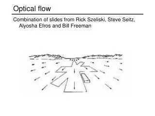
Definition of optical flow OPTICAL FLOW = apparent motion of brightness patterns Ideally, the optical flow is the projection of the three-dimensional velocity vectors on the image
Caution required ! Two examples : 1. Uniform, rotating sphere O.F. = 0 2. No motion, but changing lighting O.F. 0
Mathematical formulation I (x,y,t) = brightness at (x,y) at time t Brightness constancy assumption: Optical flow constraint equation :
Optical Flow • Brightness Constancy • The Aperture problem • Regularization • Lucas-Kanade • Coarse-to-fine • Parametric motion models • Direct depth • SSD tracking • Robust flow • Bayesian flow
The aperture problem 1 equation in 2 unknowns
What is Optic Flow, anyway? • Estimate of observed projected motion field • Not always well defined! • Compare: • Motion Field (or Scene Flow) projection of 3-D motion field • Normal Flow observed tangent motion • Optic Flow apparent motion of the brightness pattern (hopefully equal to motion field) • Consider Barber pole illusion
Optical Flow • Brightness Constancy • The Aperture problem • Regularization • Lucas-Kanade • Coarse-to-fine • Parametric motion models • Direct depth • SSD tracking • Robust flow • Bayesian flow
Horn & Schunck algorithm Additional smoothness constraint : besides OF constraint equation term minimize es+ec
so the Euler-Lagrange equations are is the Laplacian operator Horn & Schunck The Euler-Lagrange equations : In our case ,
Horn & Schunck Remarks : 1. Coupled PDEs solved using iterative methods and finite differences 2. More than two frames allow a better estimation of It 3. Information spreads from corner-type patterns
Horn & Schunck, remarks 1. Errors at boundaries 2. Example of regularisation (selection principle for the solution of illposed problems)
Optical Flow • Brightness Constancy • The Aperture problem • Regularization • Lucas-Kanade • Coarse-to-fine • Parametric motion models • Direct depth • SSD tracking • Robust flow • Bayesian flow
Optical Flow • Brightness Constancy • The Aperture problem • Regularization • Lucas-Kanade • Coarse-to-fine • Parametric motion models • Direct depth • SSD tracking • Robust flow • Bayesian flow
Optical Flow • Brightness Constancy • The Aperture problem • Regularization • Lucas-Kanade • Coarse-to-fine • Parametric motion models • Direct depth • SSD tracking • Robust flow • Bayesian flow