Understanding Optical Flow: Challenges, Approaches, and Applications in Motion Estimation
Optical flow refers to the pattern of apparent motion between images, serving as a fundamental concept in computer vision and motion estimation. This document discusses key challenges such as noise, color smoothness, lighting effects, occlusions, and abrupt movements. Various approaches are outlined, including block matching, generalized block matching, and Bayesian methods, emphasizing how they solve these challenges. Applications span video coding, segmentation, object reconstruction, and tracking. Additionally, we delve into mathematical models for 2D and 3D motion representation, ensuring a comprehensive understanding of optical flow.


Understanding Optical Flow: Challenges, Approaches, and Applications in Motion Estimation
E N D
Presentation Transcript
Optical Flow 10-24-2005
Problem • Problems in motion estimation • Noise, • color (intensity) smoothness, • lighting (shadowing effects), • occlusion, • abrupt movements, etc • Approaches: • Block matching, • Generalized block matching, • Optical flow (block-based, Horn-Schunck etc) • Bayesian, etc. • Applications • Video coding and compression, • Segmentation • Object reconstruction (structure-from-motion) • Detection and tracking, etc.
= ì x X í = y Y î Motion description • 2D motion: • p = [x(t),y(t)]p’= [x(t+ t0), y(t+t0)] • d(t) = [x(t+ t0)-x(t),y(t+t0)-y(t)] • 3D motion: • Α= [ Χ1, Υ1, Ζ1 ]ΤΒ = [ Χ2, Υ2, Ζ2 ]Τ • = R+T • Basic projection models: • Orthographic • Perspective
Optical Flow • Basic assumptions: • Image is smooth locally • Pixel intensity does not change over time (no lighting changes) • Normal flow: • Second order differential equation:
and Block-based Optical Flow Estimation • Optical flow estimation within a block (smoothness assumption): all pixels of the block have the same motion • Error: • Motion equation:
Gauss-Seidel Horn-Schunck • We want an optical flow field that satisfies the Optical Flow Equation with the minimum variance between the vectors (smoothness)