Optical Flow Methods
Optical Flow Methods. CISC 489/689 Spring 2009 University of Delaware. Outline. Review of Optical Flow Constraint, Lucas- Kanade , Horn and Schunck Methods Lucas- Kanade Meets Horn and Schunck 3D Regularization Techniques for solving optical flow Confidence Measures in Optical Flow.

Optical Flow Methods
E N D
Presentation Transcript
Optical Flow Methods CISC 489/689 Spring 2009 University of Delaware
Outline • Review of Optical Flow Constraint, Lucas-Kanade, Horn and Schunck Methods • Lucas-Kanade Meets Horn and Schunck • 3D Regularization • Techniques for solving optical flow • Confidence Measures in Optical Flow
Interpretation Constraint Line
Lucas-Kanade Method • Local Method, window based • Cannot solve for optical flow everywhere • Robust to noise Figures from Lucas/Kanade Meets Horn/Schunck: Combining Local and Global Optic Flow Methods ANDR´ES BRUHN AND JOACHIM WEICKERT, 2005
Dense optical Flow Lacks Smoothness Figures from Lucas/Kanade Meets Horn/Schunck: Combining Local and Global Optic Flow Methods ANDR´ES BRUHN AND JOACHIM WEICKERT, 2005
Horn and Schunck Method Euler-Lagrange Equations
Horn and Schunck Method • Global Method • Estimates flow everywhere • Sensitive to noise • Oversmooths the edges Figures from Lucas/Kanade Meets Horn/Schunck: Combining Local and Global Optic Flow Methods ANDR´ES BRUHN AND JOACHIM WEICKERT, 2005
Why combine them? • Need dense flow estimate • Robust to noise • Preserve discontinuities
Combined Local Global Method Euler-Lagrange Equations Table: Courtesy - Darya Frolova, Recent progress in optical flow
Preserving discontinuities • Gaussian Window does not preserve discontinuities • Solutions • Use bilateral filtering • Add gradient constancy
Bilateral support window Images: Courtesy, Darya Frolova, Recent progress in optical flow
L2: L1: xi → xi + ∆ Influence of xi on E: equal for all xi proportional to Outliers influence the most Majority decides Robust statistics – simple example Find “best” representative for the set of numbers xi Slide: Courtesy - Darya Frolova, Recent progress in optical flow
Oligarchy Democracy Robust statistics many ordinary people a very rich man wealth Votes proportional to the wealth One vote per person like in L1 norm minimization like in L2 norm minimization Slide: Courtesy - Darya Frolova, Recent progress in optical flow
usual: L2 robust regularized robust: L1 ε • easy to analyze and minimize • sensitive to outliers • robust in presence of outliers • non-smooth: hard to analyze • smooth: easy to analyze • robust in presence of outliers Combination of two flow constraints [A. Bruhn, J. Weickert, 2005] Towards ultimate motion estimation: Combining highest accuracy with real-time performance Slide: Courtesy - Darya Frolova, Recent progress in optical flow
3D Regularization • accounted for spatial regularization • If velocities do not change suddenly with time, can we regularize in time as well?
warp & upsample run iterative estimation . . . image J image I image 1 Image 2 Gaussian pyramid of image 1 Gaussian pyramid of image 2 Multiresolution estimation run iterative estimation
Multi-resolution Lucas Kanade Algorithm • Compute Iterative LK at highest level • For Each Level i • Take flow u(i-1), v(i-1) from level i-1 • Upsample the flow to create u*(i), v*(i) matrices of twice resolution for level i. • Multiply u*(i), v*(i) by 2 • Compute It from a block displaced by u*(i), v*(i) • Apply LK to get u’(i), v’(i) (the correction in flow) • Add corrections u’(i), v’(i) to obtain the flow u(i), v(i) at the ith level, i.e., u(i)=u*(i)+u’(i), v(i)=v*(i)+v’(i)
Comparison of errors For Yosemite sequence with clouds Table: Courtesy - Darya Frolova, Recent progress in optical flow
Solving the system How to solve? Start with some initial guess and apply some iterative method • fast convergence • good initial guess 2 components of success:
. . . . . . . . . . . . Relaxation smoothes the error Relaxation schemes have smoothing property: It may take thousands of iterations to propagate information to large distance Only neighboring pixels are coupled in relaxation scheme
Relaxation smoothes the error Examples 1D case: 2D case: Error of initial guess Error after 5 relaxation Error after 15 relaxations
Idea: coarser grid initial grid – fine grid On a coarser grid low frequencies become higher Hence, relaxations can be more effective coarse grid – we take every second point
Multigrid 2-Level V-Cycle 5. Correct the previous solution 6. Iterate ⇒ remove interpolation artifacts 1. Iterate ⇒error becomes smooth 2. Transfer error equation to the coarse level ⇒ low frequencies become high 4. Transfer error to the fine level 3. Solve for the error on the coarse level ⇒ good error estimation
Coarse grid - advantages Coarsening allows: • make iteration process faster (on the coarse grid we can effectively minimize the error) • obtain better initial guess (solve directly on the coarsest grid) go to the coarsest grid interpolate to the finer grid solve here the equation to find
Confidence Metric • Intrinsic in Local Methods • How to evaluate for global methods? • Edge strength? • Doesn’t work (Barron et al.,1994)
Confidence Metric • Histogram of error contribution Number of pixels Error
Further Reading • Combining the advantages of local and global optic flow methods (“Lucas/Kanade meets Horn/Schunck”) A. Bruhn, J. Weickert, C. Schnörr, 2002 - 2005 • High accuracy optical flow estimation based on a theory for warping T. Brox, A. Bruhn, N. Papenberg, J. Weickert, 2004 - 2005 • Real-Time Optic Flow Computation with Variational Methods A. Bruhn, J. Weickert, C. Feddern, T. Kohlberger, C. Schnörr, 2003 - 2005 • Towards ultimate motion estimation: Combining highest accuracy with real-time performance. A. Bruhn, J. Weickert, 2005 • Bilateral filtering-based optical flow estimation with occlusion detection. J.Xiao, H.Cheng, H.Sawhney, C.Rao, M.Isnardi, 2006