Motion estimation

1. Motion estimation Digital Visual Effects, Spring 2005 Yung-Yu Chuang 2005/3/23 with slides by Michael Black and P. Anandan

2. Announcements • Project #1 is due on next Tuesday, submission mechanism will be announced later this week. • grading: report is important, results (good/bad), discussions on implementation, interface, features, etc.

3. Outline • Motion estimation • Lucas-Kanade algorithm • Tracking • Optical flow

4. Motion estimation • Parametric motion (image alignment) • Tracking • Optical flow

5. Parametric motion

6. Tracking

7. Optical flow

8. Three assumptions • Brightness consistency • Spatial coherence • Temporal persistence

9. Brightness consistency

10. Spatial coherence

11. Temporal persistence

12. Image registration Goal: register a template image J(x) and an input image I(x), where x=(x,y)T. Image alignment: I(x) and J(x) are two images Tracking: I(x) is the image at time t. J(x) is a small patch around the point p in the image at t+1. Optical flow: I(x) and J(x) are images of t and t+1.

13. Simple approach • Minimize brightness difference

14. Simple SSD algorithm For each offset (u, v) compute E(u,v); Choose (u, v) which minimizes E(u,v); Problems: • Not efficient • No sub-pixel accuracy

15. Lucas-Kanade algorithm

16. Newton’s method • Root finding for f(x)=0 Taylor’s expansion:

17. Lucas-Kanade algorithm

18. Lucas-Kanade algorithm

19. Lucas-Kanade algorithm iterate shift I(x,y) with (u,v) compute gradient image Ix, Iy compute error image J(x,y)-I(x,y) compute Hessian matrix solve the linear system (u,v)=(u,v)+(∆u,∆v) until converge

20. translation affine Parametric model

21. minimize Parametric model minimize with respect to

22. warped image image gradient Jacobian of the warp Parametric model

23. Jacobian of the warp For example, for affine

24. Parametric model minimize Hessian

25. Lucas-Kanade algorithm iterate warp I with W(x;p) compute error image J(x,y)-I(W(x,p)) compute gradient image evaluate Jacobian at (x;p) compute compute Hessian compute solve update p by p+ until converge

27. Coarse-to-fine strategy I J refine J Jw I warp + I J Jw pyramid construction pyramid construction refine warp + J I Jw refine warp +

28. Application of image alignment

29. Tracking

30. Tracking

31. Tracking brightness constancy optical flow constraint equation

32. Optical flow constraint equation

33. Multiple constraint

34. Area-based method • Assume spatial smoothness

35. Aperture problem

36. Aperture problem

37. Aperture problem

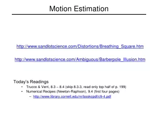
38. Demo for aperture problem • http://www.sandlotscience.com/Distortions/Breathing_objects.htm • http://www.sandlotscience.com/Ambiguous/barberpole.htm

39. Aperture problem • Larger window reduces ambiguity, but easily violates spatial smoothness assumption

40. Area-based method • Assume spatial smoothness

41. Area-based method must be invertible

42. Area-based method • The eigenvalues tell us about the local image structure. • They also tell us how well we can estimate the flow in both directions • Link to Harris corner detector

43. Textured area

44. Edge

45. Homogenous area

46. KLT tracking • Select feature by • Monitor features by measuring dissimilarity

50. KLT tracking http://www.ces.clemson.edu/~stb/klt/