3D Motion Estimation
3D Motion Estimation. 3D model construction. 3D model construction. Video Manipulation. Visual Motion. Allows us to compute useful properties of the 3D world, with very little knowledge. Example: Time to collision. Time to Collision. An object of height L moves with constant velocity v:

3D Motion Estimation
E N D
Presentation Transcript
Visual Motion • Allows us to compute useful properties of the 3D world, with very little knowledge. • Example: Time to collision
Time to Collision • An object of height L moves with constant velocity v: • At time t=0 the object is at: • D(0) = Do • At time t it is at • D(t) = Do – vt • It will crash with the camera at time: • D(t) = Do – vt = 0 • t = Do/v v L L l(t) f t t=0 Do D(t)
Time to Collision The image of the object has size l(t): v L L l(t) Taking derivative wrt time: f t t=0 Do D(t)
Time to Collision v L L l(t) f t t=0 And their ratio is: Do D(t)
Time to Collision Can be directly measured from image v L L l(t) f t t=0 And time to collision: Do D(t) Can be found, without knowing L or Do or v !!
Z u r t, Structure from Motion
Consider a 3D point P and its image: P p z f Z Using pinhole camera equation:
Let things move: V The relative velocity of P wrt camera: P v p Translation velocity Rotation angular velocity z f Z
3D Relative Velocity: V The relative velocity of P wrt camera: P v p z f Z
Motion Field: the velocity of p V P Taking derivative wrt time: v p z f Z
Motion Field: the velocity of p V P v p z f Z
Motion Field: the velocity of p V P v p z f Z
Motion Field: the velocity of p V Translational component P v p Scaling ambiguity (t and Z can only be derived up to a scale Factor) z f Z
Motion Field: the velocity of p V Rotational component P v p z f Z NOTE: The rotational component is independent of depth Z !
Pure Translation What if tz= 0 ? All motion field vectors are parallel to each other and inversely proportional to depth !
Pure Translation: Properties of the MF • If tz¹ 0 the MF is RADIAL with all vectors pointing towards (or away from) a single point po. If tz = 0 the MF is PARALLEL. • The length of the MF vectors is inversely proportional to depth Z. If tz¹ 0 it is also directly proportional to the distance between p and po.
Pure Translation: Properties of the MF • po is the vanishing point of the direction of translation. • po is the intersection of the ray parallel to the translation vector and the image plane.
Special Case: Moving Plane V Planar surfaces are common in man-made environments n P v p z f Z Question: How does the MF of a moving plane look like?
X n P d O Z Y Special Case: Moving Plane • Points on the plane must satisfy the equation describing the plane. • Let • n be the unit vector normal to the plane. • d be the distance from the plane to the origin. • NOTE: If the plane is moving wrt camera, n and dare functions of time. Then: where
Special Case: Moving Plane X be the image of P Let n Using the pinhole projection equation: P d p O Z Y Using the plane equation: Solving for Z:
X n P d p O Z Y Special Case: Moving Plane Now consider the MF equations: And Plug in:
X n P d p O Z Y Special Case: Moving Plane The MF equations become: where
X n P d p O Z Y Special Case: Moving Plane MF equations: Q: What is the significance of this? • A: The MF vectors are given by low order (second) polynomials. • Their coeffs. a1 to a8 (only 8 !) are functions of n, d, t and w. • The same coeffs. can be obtained with a different plane and relative velocity.
Moving Plane: Properties of the MF • The MF of a planar surface is at any time a quadratic function in the image coordinates. • A plane nTP=d moving with velocity V=-t-w£ P has the same MF than a plane with normal n’=t/|t| , distance d and moving with velocity V=|t|n –(w + n£ t/d)£ P
E E -urot -urot u utr utr u t Classical Structure from Motion • Established approach is the epipolar minimization: The “derotated flow” should be parallel to the translational flow.
The Translational Case(a least squares formulation) Substitute back
Step 2: Differentiate with respect to tx, ty, tz, set expression to zero. Equations are nonlinear in tx, ty, tz
Using a different norm First, differentiate integrand with respect to Z and set to zero
Differentiate g( tx, ty, tz ) with respect to tx, ty, tz and set to zero Solution is singular vector corresponding to smallest singular value
The Rotational Case Let f=1 In matrix form
The General Case Minimization of epipolar distance or, in vector notation
Motion Parallax The difference in motion between two very close points does not depend on rotation. Can be used at depth discontinuities to obtain the direction of translation. FOE
Vectors perpendicular to translational component Vector component perpendicular to translational component is only due to rotation rotation can be estimated from it.
Motion Estimation Techniques • Prazdny (1981), Burger Bhanu (1990), Nelson Aloimonos (1988), Heeger Jepson (1992): Decomposition of flow field into translational and rotational components. Translational flow field is radial (all vectors are emanating from (or pouring into) one point), rotational flow field is quadratic in image coordinates. Either search in the space of rotations: remainig flow field should be translational. Translational flow field is evaluated by minimizing deviation from radial field: . Or search in the space of directions of translation: Vectors perpendicular to translation are due to rotation only
Motion Estimation Techniques • Longuet-Higgins Prazdny (1980), Waxman (1987): Parametric model for local surface patches (planes or quadrics) solve locally for motion parameters and structure, because flow is linear in the motion parameters (quadratic or higher order in the image coordinates)