Download
1 / 29
300 likes | 384 Vues
Lucas-Kanade Motion Estimation. Thanks to Steve Seitz, Simon Baker, Takeo Kanade, and anyone else who helped develop these slides. Why estimate motion?. We live in a 4-D world Wide applications Object Tracking Camera Stabilization Image Mosaics 3D Shape Reconstruction (SFM)

E N D
Lucas-Kanade Motion Estimation Thanks to Steve Seitz, Simon Baker, Takeo Kanade, and anyone else who helped develop these slides.
Why estimate motion? • We live in a 4-D world • Wide applications • Object Tracking • Camera Stabilization • Image Mosaics • 3D Shape Reconstruction (SFM) • Special Effects (Match Move)
Key assumptions • color constancy: a point in H looks the same in I • For grayscale images, this is brightness constancy • small motion: points do not move very far • This is called the optical flow problem Problem definition: optical flow • How to estimate pixel motion from image H to image I? • Solve pixel correspondence problem • given a pixel in H, look for nearby pixels of the same color in I
Optical flow constraints (grayscale images) • Let’s look at these constraints more closely • brightness constancy: Q: what’s the equation? H(x, y) = I(x+u, y+v) • small motion: (u and v are less than 1 pixel) • suppose we take the Taylor series expansion of I:
Optical flow equation • Combining these two equations The x-component of the gradient vector. What is It ? The time derivative of the image at (x,y) How do we calculate it?
Optical flow equation • Q: how many unknowns and equations per pixel? 1 equation, but 2 unknowns (u and v) • Intuitively, what does this constraint mean? • The component of the flow in the gradient direction is determined • The component of the flow parallel to an edge is unknown • This explains the Barber Pole illusion • http://www.sandlotscience.com/Ambiguous/barberpole.htm
Solving the aperture problem • Basic idea: assume motion field is smooth • Lukas & Kanade: assume locally constant motion • pretend the pixel’s neighbors have the same (u,v) • If we use a 5x5 window, that gives us 25 equations per pixel! • Many other methods exist. Here’s an overview: • Barron, J.L., Fleet, D.J., and Beauchemin, S, Performance of optical flow techniques, International Journal of Computer Vision, 12(1):43-77, 1994.
Lukas-Kanade flow • How to get more equations for a pixel? • Basic idea: impose additional constraints • most common is to assume that the flow field is smooth locally • one method: pretend the pixel’s neighbors have the same (u,v) • If we use a 5x5 window, that gives us 25 equations per pixel!
RGB version • How to get more equations for a pixel? • Basic idea: impose additional constraints • most common is to assume that the flow field is smooth locally • one method: pretend the pixel’s neighbors have the same (u,v) • If we use a 5x5 window, that gives us 25*3 equations per pixel!
Solution: solve least squares problem • minimum least squares solution given by solution (in d) of: • The summations are over all pixels in the K x K window • This technique was first proposed by Lukas & Kanade (1981) Lukas-Kanade flow • Prob: we have more equations than unknowns
Conditions for solvability • Optimal (u, v) satisfies Lucas-Kanade equation • When is This Solvable? • ATA should be invertible • ATA should not be too small due to noise • eigenvalues l1 and l2 of ATA should not be too small • ATA should be well-conditioned • l1/ l2 should not be too large (l1 = larger eigenvalue)
Edges cause problems • large gradients, all the same • large l1, small l2
Low texture regions don’t work • gradients have small magnitude • small l1, small l2
High textured region work best • gradients are different, large magnitudes • large l1, large l2
Errors in Lukas-Kanade • What are the potential causes of errors in this procedure? • Suppose ATA is easily invertible • Suppose there is not much noise in the image • When our assumptions are violated • Brightness constancy is not satisfied • The motion is not small • A point does not move like its neighbors • window size is too large • what is the ideal window size?
Revisiting the small motion assumption • Is this motion small enough? • Probably not—it’s much larger than one pixel (2nd order terms dominate) • How might we solve this problem?
u=1.25 pixels u=2.5 pixels u=5 pixels u=10 pixels image H image I image H image I Gaussian pyramid of image H Gaussian pyramid of image I Coarse-to-fine optical flow estimation
warp & upsample run iterative L-K . . . image J image I image H image I Gaussian pyramid of image H Gaussian pyramid of image I Coarse-to-fine optical flow estimation run iterative L-K
The Flower Garden Video What should the optical flow be?
TAXI: Hamburg Taxi 256x190, (Barron 94) max speed 3.0 pix/frame LMS BA Ours Error map Smoothness error
Traffic 512x512 (Nagel) max speed: 6.0 pix/frame BA Ours Error map Smoothness error
Pepsi Can 201x201 (Black) Max speed: 2pix/frame Ours Smoothness error BA
FG: Flower Garden 360x240 (Black) Max speed: 7pix/frame BA LMS Ours Error map Smoothness error