Cost Estimation
Chapter Six. Cost Estimation. Learning Objectives. Understand the strategic role of cost estimation Understand the six steps of cost estimation Apply and understand each of three cost estimation methods: the high-low method, work measurement, and regression analysis


Cost Estimation
E N D
Presentation Transcript
Chapter Six Cost Estimation
Learning Objectives • Understand the strategic role of cost estimation • Understand the six steps of cost estimation • Apply and understand each of three cost estimation methods: the high-low method, work measurement, and regression analysis • Explain the data requirements and implementation issues associated with each estimation method
Learning Objectives (continued) • Use learning curves to estimate a certain class of non-linear cost function (i.e., to estimate costs when learning is present) • Use statistical measures to evaluate a regression analysis
Strategic Role of Cost Estimation • Cost estimation is the development of the functional relationship between a cost object and its cost drivers for the purpose of predicting the cost • Accurate cost estimates facilitate the strategic cost-management process in two ways: • Cost estimates based on activity-based, volume-based, structural, and executional cost drivers facilitate strategic positioning analysis, value-chain analysis, target costing and life-cycle costing • Knowledge of key cost drivers for a cost object, i.e., which cost drivers are most useful in predicting costs, often plays a collaborative role to judge and confirm ideas from designers and engineers
Cost Function Estimation There are six steps in the cost estimation process: • Define the cost object to be estimated • Determine the cost driver(s) • The most important step: specification of underlying causal factors of a cost • Collect consistent and accurate data • Consistent means that the data are calculated on the same accounting basis and all transactions are recorded in the proper period • Accuracy refers to the reliability of the data
Cost Function Estimation (continued) • Graph the data • To identify unusual patterns, possible nonlinearities, and any outlier observations • Select and employ a cost-estimation method (e.g., linear regression) • Assess the accuracy (descriptive validity) of the estimated cost function • One measure of the accuracy of the estimated cost function is the mean absolute percentage error (MAPE) produced by that function
Cost Estimation Methods • There are four cost estimation methods discussed in this chapter: • The High-Low method • Work measurement • Visual fit • Regression analysis (both linear and nonlinear models) • The methods above are listed in order from least to most accurate, but the cost and effort in employing the methods are the reverse of this sequence • The method chosen by the cost analyst will depend on the level of accuracy desired and any limitations on cost, time, and effort
Cost Estimation: An Example Bill Garcia, a management accountant, wants to estimate future maintenance costs for a large manufacturing company; recent monthly data are as follows:
Cost Estimation: Example (continued) Based on above information, Garcia feels that maintenance costs for August will likely be between $22,500 and $23,500, but he wants to be more accurate so he considers the use of a cost estimation method
Cost Estimation: Example (continued) That is, Garcia would like to estimate an underlying cost function for maintenance costs. Garcia feels there is an economic relationship between maintenance cost and monthly operating hours (a cost driver), so he collects the following monthly observations:
Cost Estimation: Example (continued) Another graph is created to incorporate the new data:
The High-Low Method The high-low method uses algebra to determine a unique estimation line (cost function) between representative high and low points in the data • This method provides a unique cost line rather than a rough estimate based on a visual fitting of a cost function line through a set of data points • The high-low equation is as follows:
The High-Low Method (continued) • Using the graph, Garcia picks two data points, one representative of the lower points and one representative of the higher points (these points are often, but not necessarily, the highest and lowest points in the data set) • Let us assume that Garcia picks from the data set February (low point) and April (high point) • The next step is to calculate the equation of the line connecting these two points
The High-Low Method (continued) • b = Unit variable cost = $520 ÷ 289 hours = $1.80/hour • a = Fixed cost = Total cost – Estimated variable cost • Fixed cost = $23,030 – ($1.80/hour × 3,614 hours) • Fixed cost = $23,030 – $6,505 = $16,525 • Estimated cost function: Total cost = Fixed cost + Variable cost Y = a + (b ×X)] Y = $16,525 + ($1.80 ×X)
The High-Low Method (continued) For values of the cost driver (operating hours) within the “relevant range,” the preceding equation can be used to estimate monthly maintenance costs. For example, for the month of August:
The High-Low Method (continued) Pros: • Requires less effort and cost than the other two methods • Provides a unique cost equation from which the management accountant can estimate future costs – useful in calculating total cost Cons: • Does not provide us with a measure of “goodness-of-fit” • Relies on only two points, and the selection of those two points requires judgment (that is, it discards most of the data) • The other two methods are more sophisticated and therefore will likely provide more accurate estimates of cost
Work Measurement The work-measurement method is an engineering-based estimation method that makes a detailed study of some production or service activity to measure the time or input required per unit of output • This method is applied to manufacturing operations for direct costs (i.e., where there is a strong “input-out” relationship) • This method is also used in non-manufacturing contexts to measure the time required to complete certain tasks, such as processing receipts or bills for payment
Work Measurement (continued) There are many work-measurement methods used in practice today, but work sampling is the most common • Work sampling is method that makes a series of measurements about the activity under study, and the measurements are analyzed statistically to obtain estimates of the time and/or materials the activity requires
Visual-Fit Method In the visual-fit method, the cost analyst visually fits a straight line through a plot of all of the available data, not just between the high point and the low point, making it more reliable than the high-low method.
Example of Visual Fit Cost . . . . . . . . usage
Regression Analysis Regression analysis is a statistical method for obtaining the unique cost-estimating equation by minimizing, for a set of data points, the sum of the squares of the estimation errors: • An error is the distance measured from the regression line to one of the data points • Appropriately, this method of cost-estimation is referred to as least-squares regression
Regression Analysis (continued) Regression involves two types of variables: • The dependent variable is the cost to be estimated • The independent variable is the cost driver(s) used to estimate cost: • When one cost driver is used, the regression model is referred to as a simple regression model • When two or more cost drivers are used, the regression model is referred to as a multiple regression model
Regression Analysis (continued) A simple (i.e., one-variable), linear regression equation is as follows:
Regression Analysis (continued) To illustrate a simple, linear regression cost-estimation model, the following table contains three months of data on supplies expense and production levels (normally 12 or more points will be involved): MonthSupplies Expense (Y)Production Level (X) 1 $250 50 units 2 310 100 units 3 325 150 units 4 ? 125 units
Regression Analysis (continued) 400 350 300 250 200 Regression for the data isdetermined by a statistical procedurethat finds the unique line throughthe data points, i.e., the one that minimizesthe sum of squared error distances. Supplies Expense 50 100 150 Units of Output
Regression Analysis (continued) 400 350 300 250 200 e = 15 e = 7.5 Supplies Expense e = 7.5 b = the slope of the regression line = the coefficient of the independent variableb = $0.75 variable cost per unit of output, X a = 220 Fixed Cost = $220 50 100 150 Units of Output
Regression Analysis (continued) MonthSupplies Expense (Y)Production Level (X) 1 $250 50 units 2 310 100 units 3 325 150 units 4 ? 125 units Y = a + bX Y = $220 + ($0.75 per unit 125 units) Y = $313.75 = Estimated Cost, Month 4
Regression Analysis (continued) Pros: • Objective, statistically precise method of estimating future costs • Uses all of the available data • Dummy variables can be added to the equation to represent the presence or absence of a condition (e.g., seasonality effects) • Provides quantitative measures of its precision (“goodness-of-fit”) and reliability (R-squared, t-values, the standard error of the estimate (SE), and the p-values) • Readily available software (such as Excel) to do the calculations Cons: • Can be influenced strongly by unusual data points (called outliers) resulting in a line that is not representative of most of the data • Most expensive and time-consuming method to implement
Regression Analysis: Measuring Precision and Reliability R-squared • A number between zero and one that describes the explanatory power of the regression (the degree to which the change in Y can be explained by changes in X) • A relative measure of “goodness-of-fit” (i.e., the percentage change in Y that can be explained by changes in X) • The maximum value for R² is 1.00 (i.e., 100%)
Regression Analysis: Measuring Precision and Reliability (continued) T-value • A measure of the statistical reliability of each independent variable in the cost function: does the independent variable have a valid, stable, relationship with dependent variable? • Variables with a low t-value should be evaluated and possibly removed to improve cost estimation • In a multiple-regression model, low t-values signal the possibility of multicollinearity, meaning two or more independent variables may be highly correlated with each other; removal of one or more of these variables may be desirable
Regression Analysis: Measuring Precision and Reliability (continued) Standard error of the estimate (SE) • A measure of the accuracy of the regression’s estimate • An absolute measure of “goodness-of-fit” for the regression equation (i.e., SE measures the average variability of the data points around the regression line; an SE of zero means that all of the data points are on the regression line) • Related computationally to R2 (an SE of 0 implies an R2 of 100%) • Can be used to establish Confidence Intervals for cost estimation (i.e., range estimates for future costs, based on probability assessments)
Regression Analysis: Measuring Precision and Reliability (continued) • SE can be compared to the average size of the dependent variable • If the SE value is relatively small compared to the value of the dependent variable, the regression model can be viewed as relatively “good” P-values • Measures the risk that the true (i.e., population) value of a given cost coefficient (slope) is zero; lower p-values imply rejection of the null hypothesis of no relationship between X and Y
Regression Analysis (continued) Continuing on with the Garcia example, regression software (such Excel) produces the following output:
Regression Analysis (continued) Garcia reviews the results of his analysis: • R-squared is less than 0.50, which is a bit lower than desired • However, the SE is approximately 1% of the mean of the dependent variable, which is good • The t-value on the estimated coefficient is slightly more than 2, which implies a low probability that there is no relationship between monthly maintenance costs and changes in units of output this • Associated with a marginally high t-value for the independent variable, the p-value for the regression equation is about 10% (typically, we look for a p-value of 5% or less)
Regression Analysis (continued) But why is R2 relatively low? • He notices that May’s maintenance costs are unusually low compared to the other months and decides to use a dummy variable to possibly capture seasonal effects (therefore, he assigns a value of one for May and a value of zero for the other months) • After this addition to the formula, the quantitative measures all improve: apparently, the seasonal fluctuation was distorting the results
Regression Analysis (continued) These are the results after inclusion of the dummy variable:
Data Requirements To develop a cost estimate using statistical methods (e.g., High-Low or regression analysis), management accountants must consider aspects of data collection that can significantly influence precision and reliability Which method is usually best? Regression because it is more precise and reliable Several issues arise....
Data Requirements (continued) There are three main issues: data accuracy, time period choice, and nonlinearity: • Data accuracy can be improved by strengthening internal reporting requirements and researching sources of external data • Time period choice refers to the importance of obtaining information from the same time period and for an adequate length of time • Nonlinearity can be the result of trends/seasonality, outliers, or data shifts; these events cause linear regression to be inaccurate and adjustments must be made