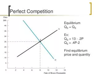
Perfect competition
Perfect competition. ECG 507 Professor Allen 9/15/05. 1. Profit Maximization. Determining the profit maximizing level of output Profit = = Total Revenue - Total Cost Total Revenue = Pq Total Cost = C(q) Therefore:. 2. Profit Maximization.

Perfect competition
E N D
Presentation Transcript
Perfect competition ECG 507 Professor Allen 9/15/05
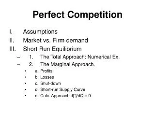
1. Profit Maximization • Determining the profit maximizing level of output • Profit = = Total Revenue - Total Cost • Total Revenue = Pq • Total Cost = C(q) • Therefore:
2. Profit Maximization • As firm expands q, TR increases with units sold • But TR increases at a decreasing rate because prices have to be cut to generate extra sales • TC increases at an increasing rate because of law of diminishing marginal returns • Expand as long as extra TR > extra TC
3. Profit Maximization • Maximize when d/dq = 0 = q(dp/dq) + p(q) – dC/dq • q(dp/dq) + p(q) = MR(q) • dC/dq = MC(q) • At q*, MR(q) = MC(q)
4. Practical considerations • Firms do not calculate MR, MC at such a fine level of detail. Focus on hours, staffing levels, overtime, orders accepted vs. declined • Careful using AVC as estimate of MC • Model is fairly general. Applies when MC constant, MC zero, and P constant
5. Output decision of competitive firm MC Price ($ per unit) 60 50 Lost profit for qq < q* Lost profit for q2 > q* D AR=MR=P 40 30 q1 : MR > MC and q2: MC > MR and q0: MC = MR but MC falling 20 10 0 1 2 3 4 5 6 7 8 9 10 11 q0 q1 q* q2 Output
At q*: MR = MC and P > ATC 6. A Competitive FirmMaking a Positive Profit MC Price ($ per unit) 60 50 A D AR=MR=P 40 ATC C B AVC 30 20 10 0 1 2 3 4 5 6 7 8 9 10 11 q0 q* Output
At q*: MR = MC and P < ATC 7. A Competitive FirmIncurring Losses MC ATC Price ($ per unit) B C D P = MR A AVC F E q* Output
8. A Competitive Firmat Zero Profits MC Price ($ per unit) 60 50 40 30 ATC AR=MR=P 20 AVC 10 6 0 1 2 3 4 5 7 8 9 10 11 Output q*
9. A Competitive FirmThat Produces Nothing MC Price ($ per unit) 60 Losses = ABCD are greater than fixed costs=AEFD. Lose less money at zero output. 50 40 ATC A D AVC 30 F E AR=MR=P 20 B C 10 6 0 1 2 3 4 5 7 8 9 10 11 Output q*
10. Choosing Output in the Short Run • Summary of Production Decisions
11. A Competitive Firm’sShort-Run Supply Curve Price ($ per unit) S = MC above AVC MC ATC P2 AVC P1 P = AVC Output q1 q2
12. Industry Supply in the Short Run The short-run industry supply curve is the horizontal summation of the supply curves of the firms. S MC1 MC2 MC3 $ per unit P3 P2 P1 5 0 2 4 7 8 10 14 21 Quantity
13. Choosing Output in the Long Run • In the long run, a firm can alter all its inputs, including the size of the plant. • We assume free entry and free exit. • Expect firms to select K so that long-run average cost is minimized
14. Output Choice in the Long Run Price ($ per unit of output) LMC LAC SMC SAC D A E $40 P = MR C B G $30 Output q1
15. Choosing Output in the Long Run • Economic profit = R - wL - rK determines whether firms enter or leave • If R > wL + rK, then firms enter • If R < wL + rK, then firms exit • If R = wL + rK, then no tendency either way
16. Long-Run Competitive Equilibrium $ per unit of output $ per unit of output Firm Industry S1 LMC $40 P1 LAC D Q1 Output Output
17. Long-Run Competitive Equilibrium $ per unit of output $ per unit of output Firm Industry S1 LMC $40 P1 LAC S2 $30 P2 D q2 Q1 Q2 Output Output
18. Choosing Output in the Long Run • Long-Run Competitive Equilibrium 1) MC = P 2) QD = QS 3) Zero economic profits • In practice firms use Economic Value Added (EVA) to make strategic decisions
19. The Industry’sLong-Run Supply Curve • To determine long-run supply, we assume all firms have access to the available production technology. • Output is increased by using more inputs, not by invention. • The shape of the long-run supply curve depends on the extent to which changes in industry output affect the prices the firms must pay for inputs.
20. Long-Run Supply in aConstant-Cost Industry Price = P1and the industry is in long-run equilibrium, P = MC = AC. $ per unit of output $ per unit of output S1 MC AC A P1 P1 D1 q1 Output Q1 Output
21. Long-Run Supply in aConstant-Cost Industry Demand increases and price increases to P2. $ per unit of output $ per unit of output S1 MC AC C P2 P2 A P1 P1 D1 D2 q1 q2 Output Q1 Output
22. Long-Run Supply in aConstant-Cost Industry Economic profits attract new firms. Supply increases to S2 and the market returns to long-run equilibrium. $ per unit of output $ per unit of output S1 S2 MC AC C P2 P2 A B P1 P1 D1 D2 q1 q2 Output Q1 Output
23. Long-Run Supply in aConstant-Cost Industry Q1 increase to Q2. Long-run supply = SL = LRAC. Change in output has no impact on input cost. $ per unit of output $ per unit of output S1 S2 MC AC C A B SL P1 P1 D1 D2 q1 Output Q1 Q2 Output
24. Increase in input prices $ per unit of output $ per unit of output S1 SMC1 LAC1 A P1 P1 D1 q1 Output Output Q1
25. Increase in input prices S3 S2 $ per unit of output $ per unit of output S1 LAC2 SMC2 SMC1 LAC1 P3 P3 P2 P2 A P1 P1 D1 q2 q1 Q3 Output Output Q1 Q2