Protein Binding Phenomena
Protein Binding Phenomena. Lecture 7, Medical Biochemstry. Ligands.

Protein Binding Phenomena
E N D
Presentation Transcript
Protein Binding Phenomena Lecture 7, Medical Biochemstry
Ligands • Ligand - any molecule that can bebound to a macromolecule (e.g., a protein). Examples of ligands include molecules ranging from small organic metabolites like glucose or ATP to large molecular polymers like glycogen or proteins. For our purposes, any molecule that can bind to a protein can be termed a ligand
Why do ligands bind proteins? • Both ligand and protein are surrounded by a water solvent shell. Each is undergoing random thermal motions that can lead to randomly oriented collisions between the protein and the ligand. Except for v. large ligands, thermally driven diffusion of the ligand is much more rapid than that of the protein.
Ligand Binding (cont) • Both protein and ligand can have functional groups such as hydroxyl, carboxyl, amino, amide and alkyl groups in various degrees of contact with the aqueous solvent. These functional groups on the ligand and on the protein may be capable of forming non-covalent bonds with each other.
Ligand Binding (cont) • If these functional groups are oriented during a collision so that they are spatially near one another, binding may occur. Of course, different ligands will have different spatial orientations of these functional groups and therefore will require different configurations of functional groups on the surface of the protein to permit binding. This matching of functional group spatial orientations are what determines the specificity of binding to that particular protein. Each protein will have its own characteristic set of binding specificities.
“Lock and Key” Binding Model For this model, the shapes of the surfaces of both protein and ligand must fit like a “lock and key”; otherwise steric hindrance will prevent binding
Induced Fit Binding Model For this model, a loosely bound ligand can interact with functional groups on the protein and cause the protein to alter its conformation so as to better fit and bind the ligand more tightly (hence induced fit). This can be thought of as a stabilization of a particular protein conformation by ligand binding.
Compare: Bond kJ/m C-C = 350 C-H = 410 O-H = 460
Scatchard Equation A mathematical model of binding phenomena
The Significance of Kd • The tighter the binding of a ligand to a protein, the smaller the Kd value (e.g. pM values) and the less likely that the ligand will dissociate from the protein once they are bound together. For a weak Kd value, the concentration is much higher (e.g., mM). These statements are made assuming that tighter binding is the desired property. Kd values are frequently used for comparisons of binding between different classes of ligands to a protein (as in comparing different drugs). Similarly, the Kd for one ligand can be compared for binding to many different receptors on the same cell or different cell types or species.
Ligand Binding Example:Intracellular Signalling Cascades • The Kd for binding of ligands (like growth factors or hormones) to their specific receptors is generally very tight with nanomolar or picomolar values. As the signalling cascade proceeds, the Kd values progressively increase (weaker binding) to micromolar values after production of cAMP. It is the very low Kd values of the receptor-ligand interactions that dictate the specificity of any signalling cascade. This is important for cellular function in that the cascades only become activated in response to specific ligand-receptor interactions.
Heme Structure Protein-Heme Complex with bound oxygen Heme-Fe2+
Myoglobin Properties • At the tertiary level, surface residues prevent one myoglobin from binding complementarily with another myoglobin; thus it only exists as a monomer. • Each monomer contains a heme prosthetic group: a protoporphryin IX derivative with a bound Fe2+ atom. • Can only bind one oxygen (O2) per monomer • The normal physiological [O2] at the muscle is high enough to saturate O2 binding of myoglobin.
Hemoglobin Properties • At the tertiary level, the surface residues of the a and b subunits form complementary sites that promote tetramer formation (a2b2), the normal physiological form of hemoglobin. • Contains 4 heme groups, so up to 4 O2 can be bound • Its physiological role is as a carrier/transporter of oxygen from the lungs to the rest of the body, therefore its oxygen binding affinity is much lower than that of myoglobin. • If the Fe2+ becomes oxidized to Fe3+ by chemicals or oxidants, oxygen can no longer bind, called Methemoglobin
Oxygen Saturation Curves • Useful analyses of myoglobin and hemoglobin functions have resulted from plotting the fraction of protein with bound O2 (fractional saturation) versus the concentration of O2 (partial pressure, p) • For myoglobin, a hyperbolic line results that reflects the high affinity of myoglobin for O2 binding • For hemoglobin, the curve is sigmoidal (S-shaped) and reflects the average affinity of the four subunits for O2 binding.
Oxygen Saturation Curves for Myoglobin & Hemoglobin
Hill Equation and Cooperativity An empirical fractional saturation equation from the oxygen curves can be derived based on the data as follows: Taking the log of this equation and rearranging results in the following Hill Equation: The slopes of the resulting straight line curves are an indication of cooperativity in binding of oxygen
The Hill Plot Cooperativity Index n = 1, no cooperativity in binding, as seen for myoglobin n > 1, positive cooperativity; binding of ligand to one subunit increases the affinity of a second site for binding, and so on, as in hemoglobin n < 1, negative cooperativity; binding of ligand to one site decreases the affinity for binding to a second site
Hemoglobin Sub-unit Types • Alpha-like (a) • 1. a : major adult form • 2. z (zeta): embyronic form • Beta-like (b) • 1. b : major adult form • 2. d : minor adult form • 3. g : major fetal form • 4. e : embyronic form Note: Complex genetic control mechanisms discussed later in the course are responsible for turning on and turning off the expression of hemoglobin during development