
Query Decomposition and Data Localization in Distributed Database Systems
E N D
Presentation Transcript
Query Decomposition AND LOCALIZATION Presented By: DarshithaBikkumalla Mohan Rakesh Dokuparthi Abhishek Reddy Regalla Instructor : Dr. Andrew Yang
OUTLINE • Query decomposition • Normalization • Reduction for vertical fragmentation. • Reduction for derived fragmentation.
Query decomposition: • Query decomposition maps a distributed calculus query into an algebraic query on global relations. • The techniques used at this layer are those of the centralized DBMS since relation distribution is not yet considered at this point. The resultant algebraic query is “good” in the sense that even if the subsequent layers apply a straightforward algorithm, the worst executions will be avoided. Data localization: • Data localization takes as input the decomposed query on global relations and applies data distribution information to the query in order to localize its data. • Data localization determines which fragments are involved in the query and thereby transforms the distributed query into a fragment query.
Query decomposition is the first phase of query processing that transforms a relational calculus query into a relational algebra query. Both input and output queries refer to global relations, without knowledge of the distribution of data. Therefore, query decomposition is the same for centralized and distributed systems. The successive steps of query decomposition are (1) Normalization, (2) Analysis, (3) Elimination of Redundancy, and (4) Rewriting. Steps 1, 3, and 4 rely on the fact that various transformations are equivalent for a given query, and some can have better performance than others.
Normalization: • The input query may be arbitrarily complex, depending on the facilities provided by the language. It is the goal of normalization to transform the query to a normalized form to facilitate further processing. With relational languages such as sql, the most important transformation is that of the query qualification (the where clause), which may be an arbitrarily complex, quantifier-free predicate, preceded by all necessary quantifiers. • There are two possible normal forms for the predicate, one giving precedence to the and (^) and the other to the or (v).
The conjunctive normal form is a conjunction (^ predicate) of disjunctions (v predicates) as follows: (P11 v p12 v.....V p1n)^......^(Pm1 v pm2 v.....V pmn) where pmn is a simple predicate. • A qualification in disjunctive normal form, on the other hand, is as follows: (P11 ^ p12 ^..... ^ p1n)v......V(pm1 ^ pm2 ^.....^ pmn)
The transformation of the quantifier-free predicate is straightforward using the well-known equivalence rules for logical operations (^, v, and ┐): 1. p1 ^ p2 ⇔ p2 ^ p1 2. p1 v p2 ⇔ p2 v p1 3. p1 ^(p2 ^ p3) ⇔(p1 ^ p2)^ p3 4. p1 v(p2 v p3) ⇔(p1 v p2)v p3 5. p1 ^(p2 v p3) ⇔(p1 ^ p2)v(p1 ^ p3) 6. p1 v(p2 ^ p3) ⇔(p1 v p2)^(p1 v p3) 7. ┐(p1 ^ p2) ⇔ ┐ p1 v ┐ p2 8. ┐(p1 v p2) ⇔ ┐ p1 ^ ┐ p2 9. ┐(┐ p) ⇔ p
In the disjunctive normal form, the query can be processed as independent conjunctive subqueries linked by unions. However, this form may lead to replicated join and select predicates. The reason is that predicates are very often linked with the other predicates by AND.
Example: “find the names of employees who have been working on project P1 for 12 or24 months” The query expressed in SQL is SELECT ENAME FROM EMP, ASG WHERE EMP.ENO = ASG.ENO AND ASG.PNO = "P1” AND DUR = 12 OR DUR = 24 The qualification in conjunctive normal form is EMP.ENO = ASG.ENO ^ ASG.PNO = “P1” ^ (DUR=12 V DUR=24) While the qualification in disjunctive normal form is (EMP.ENO = ASG.ENO ^ ASG.PNO = “P1” ^ DUR = 12) V (EMP.ENO = ASG.ENO ^ ASG.PNO = “P1” ^ DUR = 24) Treating the two conjunctions independently may lead to redundant work if common sub expressions are not eliminated.
Analysis: • Query analysis enables rejection of normalized queries for which further processing is either impossible or unnecessary. The main reasons for rejection are that the query is type incorrect or semantically incorrect. When one of these cases is detected, the query is simply returned to the user with an explanation. Otherwise, query processing is continued. • A query is type incorrect if any of its attribute or relation names are not defined in the global schema, or if operations are being applied to attributes of the wrong type. The technique used to detect type incorrect queries is similar to type checking for programming languages.
This SQL query on the engineering database is type incorrect for two reasons. First, attribute E# is not declared in the schema. Second, the operation “>200” is incompatible with the type string of ENAME. SELECT E# FROM EMP WHERE ENAME > 200
Contents • Rewriting • Transformation • Equivalence rules • Equivalent operator tree • Restructuring tree • Rewritten operator tree
Rewriting • This is the last step of query decomposition, which rewrites the query in relational algebra. • For the sake of clarity it is customary to represent the relational algebra query graphically by an operator tree. • An operator tree is a tree in which a leaf node is a relation stored in the database, and a non-leaf node is an intermediate relation produced by a relational algebra operator. • The sequence of operations is directed from the leaves to the root, which represents the answer to the query.
Transformation • The transformation of a tuple relational calculus query into an operator tree can easily be achieved as follows. • First, a different leaf is created for each different tuple variable (corresponding to a relation). In SQL, the leaves are immediately available in the FROM clause. • Second, the root node is created as a project operation involving the result attributes. These are found in the SELECT clause in SQL. • Third, the qualification (sql where clause) is translated into the appropriate sequence of relational operations (select, join, union, etc.) Going from the leaves to the root. • The sequence can be given directly by the order of appearance of the predicates and operators.
Example • “Find the names of employees other than J. Doe who worked on the CAD/CAM project for either one or two years” whose SQL expression is SELECT ENAME FROM PROJ, ASG, EMP WHERE ASG.ENO = EMP.ENO AND ASG.PNO = PROJ.PNO AND ENAME != "J. Doe” AND PROJ.PNAME = "CAD/CAM” AND (DUR = 12 OR DUR = 24)
Cont…. • The predicates have been transformed in order of appearance as join and then select operations. • By applying transformation rules, many different trees may be found equivalent to the one produced by this method. • R, s, and t are relations where r is defined over attributes a = {a1,a2, …. ,an} and s is defined over b = {b1,b2,……, bn}.
Equivalence Rules Commutativity of binary operators: • The cartesian product of two relations r and s is commutative: • Similarly, the join of two relations is commutative: • This rule also applies to union but not to set difference or semi-join.
Equivalence rules (Cont…) Associativity of binary operators : The cartesian product and the join are associative operators.
Restructing Tree • The six transformation rules are used to restructure the tree in a systematic way to eliminate “bad” operator trees. • These rules can be used in four different ways: • Firstly, they allow the separation of the unary operations, simplifying the query expression. • Second, unary operations on the same relation may be grouped. • Third, unary operations can be commuted with binary operations so that some operations may be done first. • Fourth, the binary operations can be ordered, which is used extensively in query optimization.
REDUCTION FOR VERTICAL FRAGMENTATION • The vertical fragmentation function distributes a relation based on projection attributes. • Since the reconstruction operator for vertical fragmentation is the join, the localization program for a vertically fragmented relation consists of the join of fragments on the common attributes. • Let us consider a relation emp can be divided into two vertical fragments where the key attribute eno is duplicated.
REDUCTION FOR VERTICAL FRAGMENTATION
Similar to horizontal fragmentation, queries on vertical fragments can be reduced by determining the useless intermediate relations and removing the subtrees that produce them. • Projections on a vertical fragment that has no attributes in common with the projection attributes produce useless, though not empty relations. • Let us use application related to the above statement • SELECT ENAME FROM EMP
The equivalent generic query on EMP1 AND EMP2 is given below
By commuting the projection with the join(i.E., Projecting on ENO,ENAME), we can see that the projection on EMP2 is useless because ENAME is not in EMP2.Therefore, the projection needs to apply only to EMP1
Reduction for derived fragmentation • In reduction for derived fragmentation the join of two relations is implemented as a union of partial joins. • Derived fragmentation is another way of distributing two relations so that the joint processing of select and join is improved . • Typically if relation r is subject to derived horizontal fragmentation due to relation s,the fragments of r and s that have the same join attribute values are located at the same site .
Derived fragmentation should be used only for one-to-many relationships of the form SR. • Where a tuple of s can match with n tuples of r,but a tuple of r matches with exactly one tuple of s. • Derived fragmentation can be applied to many-to-many relationships provided that tuples of s are replicated. • But such replication is difficult to maintain consistently.
Example:- reduction by derived fragmentation can be applied to the following SQL query,whichretrives all attributes of tuples from EMP and ASG that have the same value of ENO and the title “MECH.Eng” SELECT * FROM EMP,ASG WHERE ASG.ENG=EMP.ENO AND TITLE=“MECH.ENG”
The generic query on fragments EMP1,EMP2,ASG1 and ASG2 defined previously can be represented as the below figure
By pushing selection down to fragments EMP1 and emp2,the query reduces to the following query graph • This is because the selection predicate conflicts with that of emp1,and thus EMP1 can be removed.
In order to discover conflicting join predicates we distribute joins over unions and this produces the tree as follows • The left sub tree joins two fragments,asg1and emp2,whose qualifications conflict because of predicate title .Therefore left subtree can be removed .