Multidimensional Detective
Multidimensional Detective. Alfred Inselberg, Multidimensional Graphs Ltd Tel Aviv University, Israel Presented by Yimeng Dou 04-24-2002 ydou@ics.uci.edu. Parallel Coordinates.


Multidimensional Detective
E N D
Presentation Transcript
Multidimensional Detective Alfred Inselberg, Multidimensional Graphs Ltd Tel Aviv University, Israel Presented by Yimeng Dou 04-24-2002 ydou@ics.uci.edu
Parallel Coordinates • We can use parallel coordinates to model relations among multiple variables, and turn our problem into a 2-D pattern recognition problem. • It’s very useful for Visual Data Mining. • Two examples: VLSI chip and model of a country’s economy. • The model can be used to do trade-off analyses, discover sensitivities, do approximate optimizations, monitor and Decision Support.
Goals of The Program • Without any loss of information. • Low representational complexity O(N) (N is the number of dimensions). • Works for any N. • Treat every variable uniformly. • Can use transformations to recognize objects (rotation, translation, scaling, etc.). • Easily/Intuitively convey information on the properties of the N-Dimensional object. • Should be based on rigorous mathematical and algorithmic results.
In order to discover patterns from a large data set… • Must use parallel coordinates effectively, with proper geometrical understanding and queries (hence the notion of “Multidimensional Detective”). • Instead of mimicking the experience derived from standard display, a good model should exploit the special strengths of the methodology, avoids its weakness. • This task is similar to accurately cutting complicated portions of an N-dimensional watermelon. The cutting tools should be well chosen and intuitive.
The VLSI Chip Problem • Understand Figure 1—the full real data set. 473 batches, 16 processes (X1—X16). • X1—Yield (The percentage of useful chips produced in the batch). • X2—Quality (Speed performance) • X3 through X12– 10 different types of defects. 0 defect appears on top. • X13 through X16—physical parameters. • The author didn’t specify how to find high yield or high quality. I think high values appear on top, with hints from some of his later description.
Objective • Raise the yield (X1), and maintain high quality (X2). It’s a multiobjectiveoptimization problem. • It’s believed that the presence of defects hindered high yields and qualities. • So the goal is—to achieve zero defects. • (But is that really the case? ….let’s see)
Observations From Figure 2 • It isolates the batches having the highest X1 and X2. Also, notice the two clusters of X15. • It doesn’t include some batches having high X3 value (nearly 0 defects). So it casts doubt on the goal of “achieve zero defects”.Is it the right aim? • To answer this question, we construct Figure 3, which includes batches having 0 defects in at least 9 categories (they are really close to the aim of zero defects). Do they have high yields and quality?
Figure 3—Our assumption is challenged. • The nine batches have poor yields and low quality. • Here’s another visual cue—X6. The process is much more sensitive to variations in X6 than the other defects. • Treat X6 differently—select those batches with 0 X6 defects—the very best batch is included. (As shown in Figure 4).
Figure 5 and Figure 6—Test The Assumption • Figure 5 shows those batches which does not have zeros for X3 and X6. • Figure 6 shows the cluster of batches with top yields (notice there’s a gap in X1 between them and remaining batches, as seen in Figure 1). • The finding—small amounts of X3 and X6 type defects are essential for high yields and quality. • Besides, back to Fig.2, we can see X15’s relationship with X1/X2.
Our Conclusion For VLSI Chip Problem • Small ranges of X3, X6 close to (but not equal to) zero, together with the lower range of X15 provide necessary conditions for high yields and quality. • Fig.9 shows the result of constraining only X1 and the resulting gap in X15. • Fig.10 shows only constraining X2 does not yield a gap in X15.
Other Insights and The Lesson We Learned From VLSI Example • Fig.11 shows that except for two batches, the others all have very high X2. So we isolate these two batches in Fig.12—and find that the high yields but lower quality may be due to ranges of X6, X13, X14, X15. • So it suggests that we can further partition this multivariate problem into sub-problems pertaining to individual objectives.
The Economic Model Example • This example illustrates how to use interior point algorithm with the model, to do trade-off analyses, understand the impact of constraints, and in some cases do optimizations. • Interior point algorithm—We can use it to find a point that is interior to a region, and satisfies all the constraints simultaneously, so in this case, it represents a feasible economic policy for a country. • It is done interactively by sequentially choosing values of the variables. (Fig 13)
Result of Choosing The First Variable • Once a value of the first variable is chosen(Agriculture output), the dimensionality of the region is reduced by one. We can see the relationship between Agriculture and Fishing (Low ranges corresponds to each other). • So it’s possible to find a policy that favors Agriculture but not favoring Fishing and vice versa. • Mining and Fishing (see from the lower lines of Fishing in Fig.13). We find the competition between them.
Neighborhood • In Fig.15, a 20-dimensional model. The intermediate curves provide useful insights. • The steep strips in X13, X14 and X15. These 3 are critical variables, where the point is bumping the boundary.
Boundary Point and Exterior Point • Boundary point—If the polygonal line is tangent to anyone of the intermediate curves then it represents a boundary point. • Exterior point—If it crosses any intermediate curves. • Exterior point enables us to see the first variable for which the construction failed and what is needed to make corrections. • By changing variables interactively, we can discover sensitive regions and other patterns.
Before We Come To Conclusion • Is this model merely a model, or is it used (with the “intuitive” functionalities and high interactivity) in any software products? • Is this model accurate enough? • Is it sufficient to come to any conclusion about a problem using this technique when data set is very large? • How to become a skillful detective? Can any software substitute people?
Conclusion • Each multivariate dataset and problem has its own “personality” , so it requires substantial variations in the discovery scenarios and calls for considerable ingenuity ( a characteristic of a detective). • An effort of automating the exploration process is under way. It will have a number of new features, like intelligent agents, which will learn from gathered experiences.