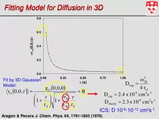
Fitting Model for Diffusion in 3D
Fit by 3D Gaussian Model:. Aragon & Pecora J. Chem. Phys. 64, 1791-1803 (1976). Fitting Model for Diffusion in 3D. ICS: D 10 -8 -10 -12 cm 2 s -1. Diffusing Population: 2D System. Simulation: D = 0.01 m m 2 s -1 ; <N>=10. Autocorrelation Function Amplitude: Number Density.

Fitting Model for Diffusion in 3D
E N D
Presentation Transcript
Fit by 3D Gaussian Model: Aragon & Pecora J. Chem. Phys. 64, 1791-1803 (1976) Fitting Model for Diffusion in 3D ICS: D 10-8-10-12 cm2s-1
Diffusing Population: 2D System Simulation: D = 0.01 mm2s-1; <N>=10 Autocorrelation Function Amplitude: Number Density Simulation: <N>=10 <N>spatial = <g(0,0)n>-1 = 10.18 ± 0.03 <N>temporal = g(0,0,0)-1 = 10.18 ± 0.01
Best Fit with 2D Diffusion Model Diffusing Population: 2D System Simulation: D = 0.01 mm2s-1; <N>=10 D2D = 0.0101 ± 0.0005mm2s-1
Flowing Population & Diffusing Population 2D Simulation: D = 0.01 mm2s-1; <N>diff =5 |v| = 0.071 mm s-1; <N>flow =5 Autocorrelation Function Amplitude: Number Density Simulation: <N>diff =5 <N>flow =5 <N>spatial = <g(0,0)n>-1 = 10.01 ± 0.03 <N>temporal : <N>diff =4.9 ± 0.3 <N>flow =5.1 ± 0.3
Best Fit with 2D Two population Diffusion & Flow Model Flowing Population & Diffusing Population 2D Simulation: D = 0.01 mm2s-1; <N>diff =5 |v| = 0.071 mm s-1; <N>flow =5 D2D = 0.010 ± 0.001mm2s-1 |v| = 0.071 ± 0.001mms-1
10 mm 2-Photon ICS on Living Cells CHO Cell: Actinin/EGFP Plated on Fibronectin Quantify Dynamics & Clustering… Two-photon fluorescence microscopy 7.5 min 37 °C
D2D = 0.0031 ± 0.0003mm2s-1 |v| = 1.12 ± 0.07mm min-1 Region 1 64x64 pixels 10% Immobile Diffusion & Flow & Immobile 3 Populations 2-Photon ICS on Living Cells 10 mm <N>Diff = 2.6 ± 0.2 mm-2 <N>flow = 0.33 ± 0.04 mm-2 <N>Immobile = 0.34 ± 0.03 mm-2
D2D = 4.7± 0.3 x10⁻⁴mm2s-1 Region 2 128x128 pixels 21% Immobile Diffusion & Immobile 2 Populations 2-Photon ICS on Living Cells 10 mm <N>Diff = 7.6 ± 0.3 mm-2 <N>Immobile = 2.0 ± 0.2 mm-2
10 m Fraction Immobile Fraction Diffusing Fraction Flowing 10 min Diffusion Dist. 10 min Flow Dist. Wiseman et al. Journal of Cell Science 117, 5521-5534, 2004 Highlighted in Nature Reviews Mol. Cell Biol. Vol 5, 953, 2004 Transport Map for a-actinin in a Living Cell
Biological Sample t=0 t=1 t=2 t=n Spatial Correlation Temporal Correlation Auto1 Auto2 Cross 2P-Image Cross-Correlation Spectroscopy (ICCS) Wiseman et al., J. Microscopy 200, 14-25 (2000)
Crosstalk Corrected Actinin - CFP 5 Integrin-YFP 2D Diffusion 2D Flow 10 mm Temporal Two-photon ICCS CHO-K1 Cells on 10 mg/mL FN Ex. 880 nm Em. 485 & 560 nm 2-Photon Imaging: 10 min, dt = 5s, 3 hr after plating
Calculate r11(x,h,t) Central Peak is r11(0,0,t) r11(0,0,t) t t=3 t=0 t=1 t=2 Spatio-Temporal Image Correlation Spectroscopy r11(x,h,t) h x Hebert et al. Biophys. J. 88-3601 (2005)
Raw Data Immobile Filtered A) B) C) Δt=15s 45s 75s 105s 135s i) ii) r(x,h,t) Hebert et al. Biophys. J. 88-3601 (2005) 1 μm r(0,0,t) Correlation Peak Tracking t t Full Space Time Correlation on Living Cells Directed Flow of a-actinin at the basal membrane
Vector Maps of a-actinin MEF Cell TIRF Microscopy Time 100 s with Images sampled at 0.1 Hz Dr. Claire Brown and Ben Hebert
9 μm/min 0 μm/min 5 μm r(x,h,t) r(x,h,t)Ff 0 s 1.5 s 2.8 s Vector Maps of a-actinin Inverse relationship b/w retrograde flow & protrusion speed (similar to actin)
Quantum Dot: Semiconductor Materials 10 nm Quantum Dots…Nanoparticles • Photostable…Different sizes…Different Colours CdSe Core ZnS Cap Surface Functionalized Silicon &Germanium Based Quantum Dots Colored Marker Tags for Molecules
20 m Dendritic Spine and Synapse Rat Purkinje neuron Particle Tracking of QD Labeled AMPA Receptors Richard Naud (Wiseman Group) with Prof. Paul DeKoninck Laval University
‘On’ state ‘Off’ state But…Quantum Dots Blink! (CdSe)ZnS – Streptavidin (QD605) TIRF Illumination CCD Detection 50ms Integration Time 2000 Frames See Bachir et al. JAP 99 (2006) Affects ICS measurements Single Dot i(t) trace Nirmal et al. Nature(London) (1996)
Some New Things: kICS k-space time correlation function 2D Fourier transform of images Point source fluorescence emitters Image series Is This Just another Acronym? No! k-space Correlation has distinct advantages… For Photobleaching and Blinking of Fluorophores Special Thanks to Prof. David Ronis See Kolin et al. Biophysical Journal 91 3061-3075 (2006)
Some New Things: kICS Intercept Photophysics Slope Transport Properties Transport Coefficients Independent of Photophysics Blinking or Photobleaching! Residuals
Some New Things: kICS Determine the slopes for each value of τ, plot them as a function of τ: Intercept D independent of wo No non-linear Curve fitting Slope t Residuals
kICS Live cell measurement a5 integrin Slope For a given :
Conclusions • Fluctuations Contain Information about Molecules • Fluctuation Size…Concentrations/Oligomerization • Fluctuation Time…Dynamics/Kinetics • FCS…Temporal Analysis of Fluctuations • Image Correlation…Space & Time Analysis • Quantum Dots…Promising…but not perfect!