The Bass Diffusion Model
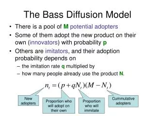
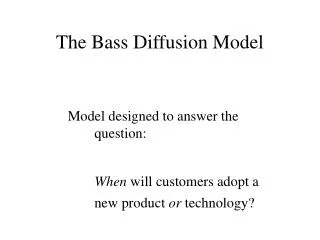
The Bass Diffusion Model. Model designed to answer the question: When will customers adopt a new product or technology?. Assumptions of the Basic Bass Model. Diffusion process is binary (consumer either adopts, or waits to adopt) Constant maximum potential number of buyers ( N )

The Bass Diffusion Model
E N D
Presentation Transcript
The Bass Diffusion Model Model designed to answer the question: When will customers adopt a new product or technology?
Assumptions of theBasic Bass Model • Diffusion process is binary (consumer either adopts, or waits to adopt) • Constant maximum potential number of buyers (N) • Eventually, all N will buy the product • No repeat purchase, or replacement purchase • The impact of the word-of-mouth is independent of adoption time • Innovation is considered independent of substitutes • The marketing strategies supporting the innovation are not explicitly included
Adoption Probability over Time (a) 1.0 Cumulative Probability of Adoption up to Time t F(t) Introduction of product Time (t) (b) f(t) = d(F(t))dt Density Function: Likelihood of Adoption at Time t Time (t)
Number of Cellular Subscribers 9,000,000 5,000,000 1,000,000 1983 1 2 3 4 5 6 7 8 9 Years Since Introduction Source: Cellular Telecommunication Industry Association
Sales Growth Model for Durables (The Bass Diffusion Model) St = p Remaining + q Adopters Potential Remaining Potential Innovation Imitation Effect Effect where: St = sales at time t p = “coefficient of innovation” q = “coefficient of imitation” # Adopters = S0 + S1 + • • • + St–1 Remaining = Total Potential – # Adopters Potential
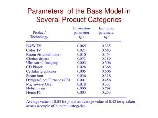
Parameters of the Bass Model in Several Product Categories Innovation Imitation Product/ parameter parameter Technology (p) (q) B&W TV 0.028 0.25 Color TV 0.005 0.84 Air conditioners 0.010 0.42 Clothes dryers 0.017 0.36 Water softeners 0.018 0.30 Record players 0.025 0.65 Cellular telephones 0.004 1.76 Steam irons 0.029 0.33 Motels 0.007 0.36 McDonalds fast food 0.018 0.54 Hybrid corn 0.039 1.01 Electric blankets 0.006 0.24 A study by Sultan, Farley, and Lehmann in 1990 suggests an average value of 0.03 for p and an average value of 0.38 for q.
Technical Specificationof the Bass Model The Bass Model proposes that the likelihood that someone in the population will purchase a new product at a particular time tgiven that she has not already purchased the product until then, is summarized by the following mathematical. Formulation Let: L(t): Likelihood of purchase at t, given that consumer has not purchased until t f(t): Instantaneous likelihood of purchase at time t F(t): Cumulative probability that a consumer would buy the product by time t Once f(t) is specified, then F(t) is simply the cumulative distribution of f(t), and from Bayes Theorem, it follows that: L(t) = f(t)/[1–F(t)] (1)
Technical Specificationof the Bass Model cont’d The Bass model proposes that L(t) is a linear function: q L(t) = p + –– N(t) (2) N where p = Coefficient of innovation (or coefficient of external influence) q = Coefficient of imitation (or coefficient of internal influence) N(t) = Total number of adopters of the product up to time t N = Total number of potential buyers of the new product Then the number of customers who will purchase the product at time t is equal to Nf(t) . From (1), it then follows that: q Nf(t) = [ p + –– N(t)][1 – N(t)] (3) N Nf(t) may be interpreted as the number of buyers of the product at time t [ = (t)]. Likewise, NF(t ) is equal to the cumulative number of buyers of the product up to time t [ = N(t)].
Bass Model cont’d Noting that [n(t) = Nf(t)] is equal to the number of buyers at time t, and [N(t) = NF(t)] is equal to the cumulative number of buyers until time t, we get from (2): q Nf(t) = [ p + –– N(t)][1 – N(t)] (3) N After simplification, this gives the basic diffusion equation for predicting new product sales: q n (t) = pN + (q – p) [N(t)] – –– [N(t)]2 (4) N
Estimating the Parameters of the Bass Model Using Non-Linear Regression An equivalent way to represent N(t) in the Bass model is the following equation: q n(t) = p + –– N(t–1) [N – N(t–1)] N Given four or more values of N(t) we can estimate the three parameters of the above equation to minimize the sum of squared deviations.
Estimating the Parameters of the Bass Model Using Regression The discretized version of the Bass model is obtained from (4): n(t) = a + bN(t–1) + cN 2(t–1) a, b, and c may be determined from ordinary least squares regression. The values of the model parameters are then obtained as follows: –b – b2 – 4ac N = –––––––––––––– 2c a p = –– N q = p + b To be consistent with the model, N > 0, b 0, and c < 0.
Forecasting Using the Bass Model—Room Temperature Control Unit Cumulative Quarter Sales Sales Market Size = 16,000 (At Start Price) 0 0 0 1 160 160 Innovation Rate = 0.01 4 425 1,118 (Parameter p) 8 1,234 4,678 12 1,646 11,166 Imitation Rate = 0.41 16 555 15,106 (Parameter q) 20 78 15,890 24 9 15,987 Initial Price = $400 28 1 15,999 32 0 16,000 Final Price = $400 36 0 16,000 Example computations n(t) = pN + (q–p) N(t–1) – qN(t–1) 2/N Sales in Quarter 1 = 0.01 16,000 + (0.41–0.01) 0 – (0.41/16,000) (0)2 = 160 Sales in Quarter 2 = 0.01 16,000 + (0.40) 160 – (0.41/16,000) (160)2 = 223.35
Factors Affecting theRate of Diffusion Product-related • High relative advantage over existing products • High degree of compatibility with existing approaches • Low complexity • Can be tried on a limited basis • Benefits are observable Market-related • Type of innovation adoption decision (eg, does it involve switching from familiar way of doing things?) • Communication channels used • Nature of “links” among market participants • Nature and effect of promotional efforts
Some Extensions to the Basic Bass Model • Varying market potential As a function of product price, reduction in uncertainty in product performance, and growth in population, and increases in retail outlets. • Incorporation of marketing variables Coefficient of innovation (p) as a function of advertising p(t) = a + b ln A(t). Effects of price and detailing. • Incorporating repeat purchases • Multi-stage diffusion process Awareness Interest Adoption Word of mouth
Pretest Market Models • Objective Forecast sales/share for new product before a real test market or product launch • Conceptual model Awareness xAvailability xTrial x Repeat • Commercial pre-test market services • Yankelovich, Skelly, and White • Bases • Assessor
ASSESSOR Model Objectives • Predict new product’s long-term market share, and sales volume over time • Estimate the sources of the new product’s share, which includes “cannibalization” of the firm’s existing products, and the “draw” from competitor brands • Generate diagnostics to improve the product and its marketing program • Evaluate impact of alternative marketing mix elements such as price, package, etc.
Consumer Research Input (Laboratory Measures) (Post-Usage Measures) Management Input (Positioning Strategy) (Marketing Plan) Preference Model Trial & Repeat Model Reconcile Outputs Draw & Cannibalization Estimates Brand Share Prediction Unit Sales Volume Diagnostics Overview of ASSESSORModeling Procedure
Overview of ASSESSOR Measurements Design Procedure Measurement O1 Respondent screening and Criteria for target-group identification recruitment (personal interview) (eg, product-class usage) O2 Pre-measurement for established Composition of ‘relevant set’ of brands (self-administrated established brands, attribute weights questionnaire) and ratings, and preferences X1 Exposure to advertising for established brands and new brands [O3] Measurement of reactions to the Optional, e.g. likability and advertising materials (self- believability ratings of advertising administered questionnaire) materials X2 Simulated shopping trip and exposure to display of new and established brands O4 Purchase opportunity (choice recorded Brand(s) purchased by research personnel) X3 Home use/consumption of new brand O5 Post-usage measurement (telephone New-brand usage rate, satisfaction ratings, and repeat-purchase propensity; attribute ratings and preferences for ‘relevant set’ of established brands plus the new brand O = Measurement; X = Advertsing or product exposure
Trial/Repeat Model Market share for new product Mn = T´R´W where: T = long-run cumulative trial rate (estimated from measurement at O4) R = long-run repeat rate (estimated from measurements at O5) W = relative usage rate, with w = 1 being the average market usage rate.
Trial Model T = FKD + CU – (FKD)´ (CU) where: F = long-run probability of trial given 100% awareness and 100% distribution (from O4) K = long-run probability of awareness (from managerial judgment) D = long-run probability of product availability where target segment shops (managerial judgment and experience) C = probability of consumer receiving sample (Managerial judgment) U = probability that consumer who receives a product will use it (from managerial judgment and past experience)
Repeat Model Obtained as long-run equilibrium of the switching matrix estimated from (O2 and O5): Time (t+1) New Other New p(nn) p(no) Time t Other p(on) p(oo) p(.) are probabilities of switching where p(nn) + p(no) = 1.0; p(on) + p(oo) = 1.0 Long-run repeat given by: p(on) r = –––––––––––––– 1 + p(on) – p(nn)
Preference Model: Purchase Probabilities Before New Product Use (Vij)b Lij = –––––––– Ri å (Vik)b k=1 where: Vij = Preference rating from product j by participant i Lij= Probability that participant i will purchase product j Ri = Products that participant i will consider for purchase (Relevant set) b = An index which determines how strongly preference for a product will translate to choice of that product (typical range: 1.5–3.0)
Preference Model: Purchase Probabilities After New Product Use (Vij)b L´ij = ––––––––––––––––– Ri (Vin)b + å (Vik)b k=1 where: L´it = Choice probability of product j after participant i has had an opportunity to try the new product b = index obtained earlier Then, market share for new product: L´inM´n = Enå –––IN n = index for new product En = proportion of participants who include new product in their relevant sets N = number of respondents
Estimating Cannibalizationand Draw Partition the group of participants into two: those who include new product in their consideration sets, and those who don’t. The weighted pre- and post- market shares are then given by: LinMj = å ––– IN L´inL´inM´j = Enå ––– + (1 – En)å ––– IN IN Then the market share drawn by the new product from each of the existing products is given by: Dj = Mj – M´j
Example: Preference Ratings Vij (Pre-use) V´ij (Post-use) Customer B1 B2 B3 B4 B1 B2 B3 B4 New Product 1 0.1 0.0 4.9 3.7 0.1 0.0 2.6 1.7 0.2 2 1.5 0.7 3.0 0.0 1.6 0.6 0.6 0.0 3.1 3 2.5 2.9 0.0 0.0 2.3 1.4 0.0 0.0 2.3 4 3.1 3.4 0.0 0.0 3.3 3.4 0.0 0.0 0.7 5 0.0 1.3 0.0 0.0 0.0 1.2 0.0 0.0 0.0 6 4.1 0.0 0.0 0.0 4.3 0.0 0.0 0.0 2.1 7 0.4 2.1 0.0 2.9 0.4 2.1 0.0 1.6 0.1 8 0.6 0.2 0.0 0.0 0.6 0.2 0.0 0.0 5.0 9 4.8 2.4 0.0 0.0 5.0 2.2 0.0 0.0 0.3 10 0.7 0.0 4.9 0.0 0.7 0.0 3.4 0.0 0.9
Choice Probabilities Lij (Pre-use) L´ij (Post-use)Customer B1 B2 B3 B4 B1 B2 B3 B4 New Product 1 0.00 0.00 0.63 0.37 0.00 0.00 0.69 0.31 0.00 2 0.20 0.05 0.75 0.00 0.21 0.03 0.03 0.00 0.73 3 0.43 0.57 0.00 0.00 0.42 0.16 0.00 0.00 0.42 4 0.46 0.54 0.00 0.00 0.47 0.50 0.00 0.00 0.03 5 0.00 1.00 0.00 0.00 0.00 1.00 0.00 0.00 0.00 6 1.00 0.00 0.00 0.00 0.80 0.00 0.00 0.00 0.20 7 0.01 0.35 0.00 0.64 0.03 0.61 0.00 0.36 0.00 8 0.89 0.11 0.00 0.00 0.02 0.00 0.00 0.00 0.98 9 0.79 0.21 0.00 0.00 0.82 0.18 0.00 0.00 0.00 10 0.02 0.00 0.98 0.00 0.04 0.00 0.89 0.00 0.07 Unweighted market share (%) 38.0 28.3 23.6 10.1 28.1 24.8 16.1 6.7 24.3 New product’s draw from each brand (Unweighted %) 9.9 3.5 7.5 3.4 New product’s draw from each brand (Weighted by En in %) 2.0 0.7 1.5 0.7
Long-term market share from advertising 0.39 Assessor Trial & Repeat Model Market Share Due to Advertising Response Mode Manual Mode % making first purchase GIVEN awareness & availability 0.23 Prob. of awareness 0.70 Prob. of availability 0.85 Prob. of switching TO brand 0.16 Prob. of repurchase of brand 0.60 • Max trial with • unlimited Ad • Ad$ for 50% • max. trial • Actual Ad $ • Max awareness • with unlimited Ad • Ad $ for 50% • max. awareness • Actual Ad $ % buying brand in simulated shopping Awareness estimate Distribution estimate (Agree) Switchback rate of non-purchasers Repurchase rate of simulation purchasers % making first purchase due to advertising 0.137 Retention rate GIVEN trial for ad purchasers 0.286 Source: Thomas Burnham, University of Texas at Austin
Correction for sampling/ad overlap (take out those who tried sampling, but would have tried due to ad) 0.035 Market share trying samples 0.251 Long-term market share from sampling 0.02 Assessor Trial & Repeat Model Market Share Due to Sampling Sampling coverage (%) 0.503 % Delivered 0.90 % of those delivered hitting target 0.80 Simulation sample use Switchback rate of non-purchasers Repurchase rate of simulation non-purchasers % hitting target that get used 0.60 Prob. of switching TO brand 0.16 Prob. of repurchase of brand 0.427 Retention rate GIVEN trial for sample receivers 0.218 Source: Thomas Burnham, University of Texas at Austin
Draw & cannibalization calculations Assessor Preference Model Summary Pre-use preference ratings Pre-use choices Post-use preference ratings Proportion of consumers who consider product 0.137 Pre-entry market shares Post-entry market shares (assuming consideration 0.274 Weighted post entry market shares 0.038 Beta (B) for choice model Pre-use constant sum evaluations Post-use constant sum evaluations Cumulative trial from ad (T&R model) 0.137 Source: Thomas Burnham, University of Texas at Austin
Market share 0.059 Market size 60M Sales per person $5 JWC factory sales 16.7 Average unit margin 0.541 Ad/sampling expense 4.5/3.5 JWC factory sales Industry average sales $ for market share 17.7 Unit-dollar adjustment 0.94 Frequency of use differences 0.9 Price differences 1.04 Net contribution JWC factory sales 16.7 Return on sales Assessor Market Share to Financial Results Diagrams Source: Thomas Burnham, University of Texas at Austin
Predicted and Observed Market Shares for ASSESSOR Deviation Deviation Product Description Initial Adjusted Actual (Initial – (Adjusted – Actual) Actual) Deodorant 13.3 11.0 10.4 2.9 0.6 Antacid 9.6 10.0 10.5 –0.9 –0.5 Shampoo 3.0 3.0 3.2 –0.2 –0.2 Shampoo 1.8 1.8 1.9 –0.1 –0.1 Cleaner 12.0 12.0 12.5 –0.5 –0.5 Pet Food 17.0 21.0 22.0 –5.0 –1.0 Analgesic 3.0 3.0 2.0 1.0 1.0 Cereal 8.0 4.3 4.2 3.8 0.1 Shampoo 15.6 15.6 15.6 0.0 0.0 Juice Drink 4.9 4.9 5.0 –0.1 –0.1 Frozen Food 2.0 2.0 2.2 –0.2 –0.2 Cereal 9.0 7.9 7.2 1.8 0.7 Etc. ... ... ... ... ... Average 7.9 7.5 7.3 0.6 0.2 Average Absolute Deviation — — — 1.5 0.6 Standard Deviation of Differences — — — 2.0 1.0
BASES Model Trial volume estimate Calibrated Distribution Awareness Pt = ´´ intent score intensityt levelt Tt = Pt ´ U0´ (1/Sit) ´ (TM) ´ (1/CDI) where: Pt = Cumulative penetration up to time t Tt = Total trial volume until time t in a particular target market U0 = Average units purchased at trial (t = 0) Sit = Seasonality index at time = t TM = Size of target market CDI = Category development index for target market
BASES Model cont’d Repeat volume estimate ¥ Rt = åNi–1,tYit Ui i=1 where: Ni–1,t = Cumulative number of consumers who repeat at least i–1 times by week t (N0,t= initial trial volume) Yit = Conditional cumulative ith repeat purchase rate at week t given that i–1 repeat purchases were made up to week t Ui = Average units purchased at repeat level i Ni–1,t & Yit are estimated based on consumers’ stated “after use intended purchase frequency” and estimate of long-run decay in repeat rate. Ui is estimated based on consumers’ stated purchase quantities.
BASES Model cont’d Total volume estimate St = Tt ´Rt + Adjustments for promotional volume
Yankelovich, Skelly and White Model Forecast market share = S ´ N ´ C ´ R ´ U ´ K where: S = Lab store sales (indicator of trial), N = Novelty factor of being in lab market. Discount sales by 20–40% based on previous experience that relate trial in lab markets to trial in actual markets, C = Clout factor which retains between 25% and 75% of SN determined, based on proposed marketing effort versus ad and distribution weights of existing brands in relation to their market share, R = Repurchase rate based on percentage of those trying who repurchase, U = Usage rate based on usage frequency of new product as compared to the new product category as a whole, and K = Judgmental factor based on comparison of S ´ N ´ C ´ R ´ U´ K with Yankelovich norms. The comparison is with respect to factors such as size and growth of category, new product’s share derived from category expansion versus conversion from existing brand.
Some Issues in ValidatingPre-Test Models • Validation does not include products that were withdrawn as a result of model predictions • Pre-test and actual launch are separated in time, often by a year or more • Marketing program as implemented could be different from planned program