Download
1 / 35
350 likes | 471 Vues
This document explores the logic and application of One-Way Analysis of Variance (ANOVA) with a single independent variable in a between-subjects design. It details hypothesis formulation, variability measures, the statistical F-ratio, and significance testing, particularly in the context of experimental research, such as the effects of epinephrine on memory and treatment efficacy in PTSD. Key statistical calculations, including degrees of freedom and mean squares, are presented alongside summary tables and tentative conclusions, addressing the implications of findings and potential for multiple comparisons.

E N D
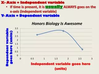
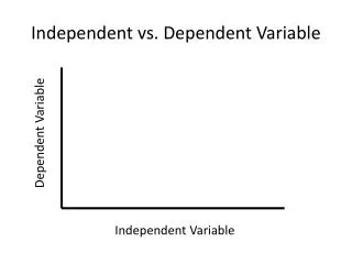
One-way Analysis of Variance Single Independent Variable Between-Subjects Design
Logic of the Analysis of Variance • Null hypothesis H0 : Population means equal • m1 = m2 = m3 = m4 • Alternative hypothesis: H1 • Not all population means equal. Cont.
Logic--cont. • Create a measure of variability among group means • Msgroups(accurate est. of pop. var. if null true) • Create a measure of variability within groups • MSerror(accurate est. of pop. var. regardless of whether null is true) Cont.
Logic--cont. • Form ratio of MSgroups /MSerror • Ratio approximately 1 if null true • Ratio significantly larger than 1 if null false • “approximately 1” can actually be as high as 2 or 3, but not much higher
Epinephrine and Memory • Based on Introini-Collison & McGaugh (1986) • Trained mice to go left on Y maze • Injected with 0, .1, .3, or 1.0 mg/kg epinephrine • Next day trained to go right in same Y maze • dep. Var. = # trials to learn reversal • More trials indicates better retention of Day 1 • Reflects epinephrine’s effect on memory
Calculations • Start with Sum of Squares (SS) • We need: • SStotal • SSgroups • SSerror • Compute degrees of freedom (df) • Compute mean squares and F Cont.
Degrees of Freedom (df ) • Number of “observations” free to vary • dftotal = N - 1 • Variability of N observations • dfgroups = g - 1 • variability of g means • dferror = g (n - 1) • n observations in each group = n - 1 df • times g groups
Conclusions • The F for groups is significant. • We would obtain an F of this size, when H0 true, less than one time out of 1000. • The difference in group means cannot be explained by random error. • The number of trials to learn reversal depends on level of epinephrine. Cont.
Conclusions--cont. • The injection of epinephrine following learning appears to consolidate that learning. • High doses may have negative effect.
Unequal Sample Sizes • With one-way, no particular problem • Multiply mean deviations by appropriate ni as you go • The problem is more complex with more complex designs, as shown in next chapter. • Example from Foa, Rothbaum, Riggs, & Murdock (1991)
Post-Traumatic Stress Disorder • Four treatment groups given psychotherapy • Stress Inoculation Therapy (SIT) • Standard techniques for handling stress • Prolonged exposure (PE) • Reviewed the event repeatedly in their mind Cont.
Post-Traumatic Stress Disorder--cont. • Supportive counseling (SC) • Standard counseling • Waiting List Control (WL) • No treatment
SIT = Stress Inoculation Therapy PE = Prolonged Exposure SC = Supportive Counseling WL = Waiting List Control Grand mean = 15.622
Tentative Conclusions • Fewer symptoms with SIT and PE than with other two • Also considerable variability within treatment groups • Is variability among means just a reflection of variability of individuals?
Calculations • Almost the same as earlier • Note differences • We multiply by nj as we go along. • MSerror is now a weighted average. Cont.
Summary Table F.05(3,41) = 2.84
Conclusions • F is significant at a = .05 • The population means are not all equal • Some therapies lead to greater improvement than others. • SIT appears to be most effective.
Multiple Comparisons • Significant F only shows that not all groups are equal • We want to know what groups are different. • Such procedures are designed to control familywise error rate. • Familywise error rate defined • Contrast with per comparison error rate
More on Error Rates • Most tests reduce significance level (a) for each t test. • The more tests we run the more likely we are to make Type I error. • Good reason to hold down number of tests
Fisher’s LSD Procedure • Requires significant overall F, or no tests • Run standard t tests between pairs of groups. • Often we replace s 2j or pooled estimate with MSerror from overall analysis • It is really just a pooled error term, but with more degrees of freedom--pooled across all treatment groups.
Bonferroni t Test • Run t tests between pairs of groups, as usual • Hold down number of t tests • Reject if t exceeds critical value in Bonferroni table • Works by using a more strict value of a for each comparison Cont.
Bonferroni t--cont. • Critical value of a for each test set at .05/c, where c = number of tests run • Assuming familywise a = .05 • e. g. with 3 tests, each t must be significant at .05/3 = .0167 level. • With computer printout, just make sure calculated probability < .05/c • Necessary table is in the book
Assumptions for Anal. of Var. • Assume: • Observations normally distributed within each population • Population variances are equal • Homogeneity of variance or homoscedasticity • Observations are independent Cont.
Assumptions--cont. • Analysis of variance is generally robust to first two • A robust test is one that is not greatly affected by violations of assumptions.
Magnitude of Effect • Eta squared (h2) • Easy to calculate • Somewhat biased on the high side • Formula • See slide #33 • Percent of variation in the data that can be attributed to treatment differences Cont.
Magnitude of Effect--cont. • Omega squared (w2) • Much less biased than h2 • Not as intuitive • We adjust both numerator and denominator with MSerror • Formula on next slide
h2 and w2 for Foa, et al. • h2 = .18: 18% of variability in symptoms can be accounted for by treatment • w2 = .12: This is a less biased estimate, and note that it is 33% smaller.
Other Measures of Effect Size • We can use the same kinds of measures we talked about with t tests. • Usually makes most sense to talk about 2 groups at a time, rather than a measure averaged over several groups.
Darley & Latene (1968) Condition: Alone One Other Four Others n 13 26 13 X .87 .72 .51